Microeconomics
Macroeconomics
SISTERetrics
SITES
Compleat World Copyright Website
World Cultural Intelligence Network
Dr. Harry Hillman Chartrand, PhD
Cultural Economist & Publisher
©
h.h.chartrand@compilerpress.ca
215 Lake Crescent
Saskatoon, Saskatchewan
Canada,
S7H 3A1
Launched 1998
|
Macroeconomics 4.0 Aggregate Supply & Equilibrium
|
|
Aggregated
output or supply
Ys = f (K, L, N, .....) where: Ys = aggregate supply; f = some function of technology or 'know-how'; K = Capital; L = Labour; N = Natural Resources; and, ... = all other imaginable factors of production or inputs.
Taken together, available Capital, Labour and Natural Resources constitute
The definition of capital is an unresolved problem in economics. To Marxists, it is theft. To the mainstream, its definition remains problematic as noted by T.K. Rymes of Carleton University in conversation with the author in the early 1970s: “If there is no theory of capital, there is no economics. And there is no theory of capital!” Actually there are many. Today, when economists speak of Capital, they may refer to cultural, financial, human, legal, physical, social or other forms expressed as a stock, e.g., the physical plant and equipment existing at a given moment in time. For our purposes Capital is so defined: physical plant and equipment existing at a given moment in time. Financial capital is treated, for our purposes, as money acting as a unit of account for this physical capital. There are three forms of Labour: Productive, Managerial & Entrepreneurial. All three embody personal knowledge. Productive workers are those on the shop floor actually producing goods & services. They are concerned with output. Their knowledge is technical and specialized to a given industry or firm. In this sense the competitiveness of a firm or nation “depends not only on sensible decisions about what to do, but on the availability of the skills that are required to do it” (Loasby 1998, 143). Management, among other things, means “a governing body of an organization or business, regarded collectively; the group of employees which administers and controls a business or industry, as opposed to the labour force”. The role of management is to make available the means (inputs) so production workers can perform their tasks and then market and distribute the output. One crucial characteristic of the firm is custom including tacit understandings of entitlements and obligations between productive, managerial and entrepreneurial workers. This constitutes part of ‘corporate culture’. With the notable exception of firms like Microsoft (Bill Gates) and Walmart (Sam Walton), most major corporations do not follow an original founder/owner but rather a ‘hired gun’, or business entrepreneur. The word ‘entrepreneur’ comes from the French entre meaning ‘between’ and prendre meaning ‘to take’. The English ‘middleman’ retains this original sense. Today the term usually refers to someone who sees and seizes an economic opportunity or a market opening or gap. This may take the form of a new product or of servicing an existing market in a new way. In both cases a high degree of creativity and risk-taking is implicit. Entrepreneurial knowledge is intuitive in seeing and taking advantage of invariants and affordances in a market that others do not see. It involves seeing and realizing a vision of future markets, products and opportunities and leads the organization in realizing that vision. Similarly, the definition of a natural resources is constantly evolving. At first glance, natural resources have no relationship to knowledge. By definition, they exist as John Locke said in “the State that Nature hath provided”. They are just part of the environment until the knowing mind recognizes them as useful. Thus oil lay in the ground virtually untapped until invention of the internal combustion engine. Just as we recognize a tool by its purpose, we similarly identify natural resources by the human ends we attribute to them. At a given point in time a naturally occurring substance is seen as nothing but an environmental feature. Take a pathway through the jungle one day and you see a large rock outcrop. The next day, with new knowledge, the same path leads not to an environmental feature but to a bauxite deposit that can be converted into aluminum. It has become a toolable natural resource. Yet it itself has not changed, one day to the next, rather new knowledge allows us to see it in a different light. What do we mean by technology? The word ‘technology’ entered the English language only in 1859 according to the Merriam Webster Dictionary deriving from the Greek techne meaning Art and logos meaning Reason, i.e., reasoned art. Physical technology, to paraphrase Heidegger, is the enframing and enabling of Nature to serve human purpose. Technological change in the Standard Model of Market Economics refers to the impact of new knowledge on the production function of a firm or nation. The content and source of that knowledge is not a theoretical concern; what matters is its mathematical impact on the production function.
Existing business models can be overturned by technological change, e.g., information technology in the 1980s reduced the need for middle management and resulted in significant 'downsizing' of large firms. In response to technological change, the production function may shift upwards or downwards, i.e., technology can be lost as well as found, e.g., after the fall of Roman Empire. The quantity and/or cost per unit output may increase or decrease. Alternatively, an entirely new production function may emerge with innovation of new and/or elimination of old products, processes and techniques. Technological knowledge thus does not only accumulate; it also withers away if not transmitted to subsequent generations. The later is most apparent with respect to traditional craft methods (White & Hart 1990) and arguably with deindustrialization of many parts of the developed world. The process has been compared by Kaufmann to speciation and extinction in biology (Kauffman 2000 216). 4.2 Short Run Aggregate Supply (SAS) (MKM C14/352-6: 329-33; 338-341) We will derive both Aggregate Supply Curves - Short Run (SAS) and Long Run (LAS) - using what Keynes called "diagrammatic illustrations of economic problems" (Keynes 1924, 329). As with Aggregate Expenditure and Demand there are, on the supply side of the macroeconomic equation, two supply curves - the short-run aggregate supply (SAS) and the long-run or potential aggregate supply (LAS) . This results in the 'Keynesian double cross'. In Microeconomics, X marks the spot of market equilibrium of Supply and Demand. In Macroeconomics there are two Supply and two Demand curves and equilibrium is defined with respect to both the current (short run) and potential (long run) equilibrium of a national economy.
SAS is plotted using
the schedule of increasing price levels (Y axis) and real GDP (X axis)
(P&B
7th Ed Fig. 26.1;
R&L 13th Ed
Fig. 23-4;
MKM Fig. 14.7) assuming nominal factor prices remain
constant. This means that if the overall price level rises then real
factor prices decline resulting in increased production.
There is, however, within the economics profession, controversy about SAS's slope. Thus in the Classical Model it is assumed that money wages and prices are perfectly flexible. This means any increase in demand simply raises prices rather than expand output. SAS is inelastic or even vertical. It is with this assumption that Keynes took exception. He believed that the money wage was not perfectly flexible. Rather, it was subject to at least four rigidities . First, wage bargaining tends to focus not just on the wage rate but also on the wage differential between different types of workers, i.e., there is no an homogenous unit of Labour but rather many different forms and types. A given group of workers resist wage cuts not just because of the financial cost but also the status implications relative to other workers. A case in point is the wage differential between police officers and fire fighters. Over time a wage differential develops reflecting the relative worth of each group. Any attempt to alter that balance tends to be resisted. Second, unions negotiate contracts for specific time periods, e.g., two or three years. During that period the money wage cannot be changed by firms. Third, even when there is no formal contract between unions and firms there is a tendency – a convention - to maintain the money wage for a given time period. Fourth, Labour exhibits 'backward looking expectations' about price changes, a.k.a., inflation. Thus they expect the future to be a projection of past experience. Business, on the other hand, exhibits 'forward looking expectations' given its day-to-day experience of the changing prices of inputs, outputs and competitors. Taken together these four factors make the money wage ‘sticky’ rather than perfectly flexible as assumed in the Classical Model and in the New Classical Model known as the School of Rational Expectations. Under the Keynesian Model 'sticky' wages results in a SAS curve with a relatively gentle upward slope. In the Classical and New Classical Models, flexible wages and prices result in a very inelastic or even vertical SAS. The difference in the slope of the SAS curve has significant implications for fiscal and monetary policy. 4.3 Long Run/Potential Aggregate Supply (LAS) (MKM C14/347-50: 324-27; 334-336)
The Long Run
Aggregate Supply Curve (LAS) is found when all available factors of
production (K, L, N, T, etc.) are fully employed (P&B
7th Ed Fig. 26.1;
MKM Fig. 14.5). LAS is vertical meaning there can be no increase in
output given that factors of production are fully employed. LAS
corresponds to potential real GDP of a national economy, that is, the
maximum output attainable given the existing supply of factors of
production.
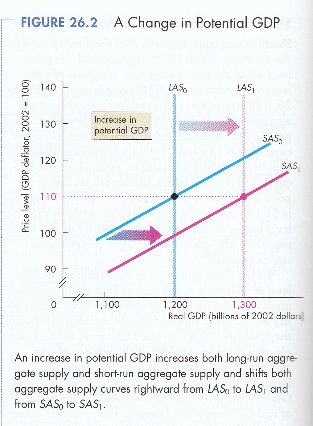
LAS can shift, left or right, if there are increases or decreases in available factors of production, e.g. the quantity of labour grows or shrinks, changes in the quantity of capital (investment) or technological progress (P&B 7th Ed 26.2; R&L 13th Ed Fig. 24-5; MKM Fig. 14.6). In this regard it is important to realize that technological knowledge can be lost as well as found. Take the case of the Roman Empire after the barbarian conquest.
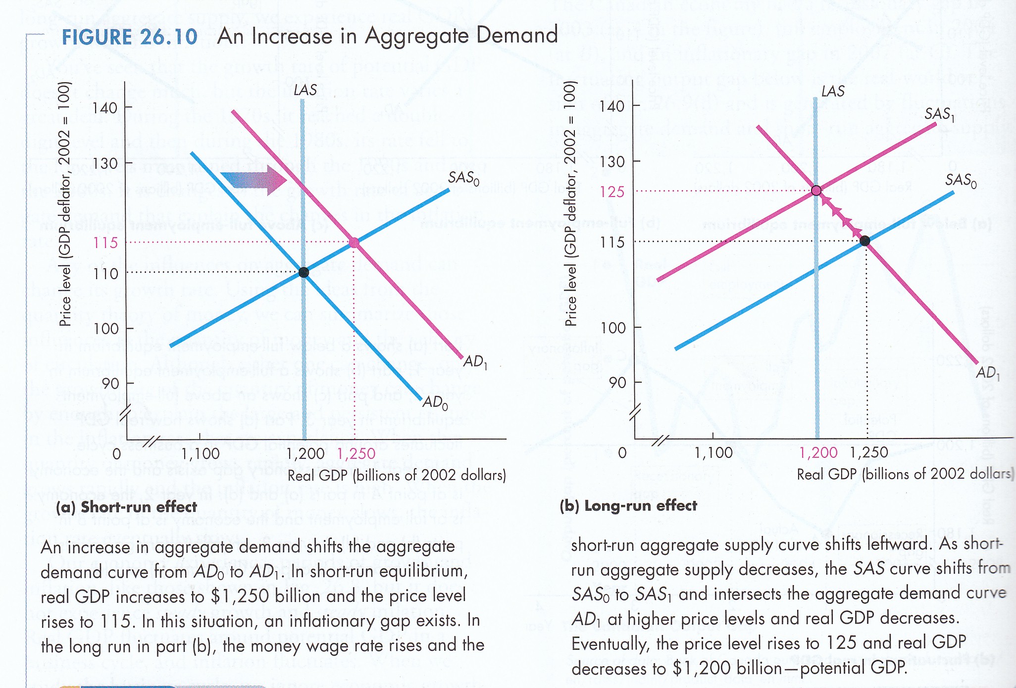
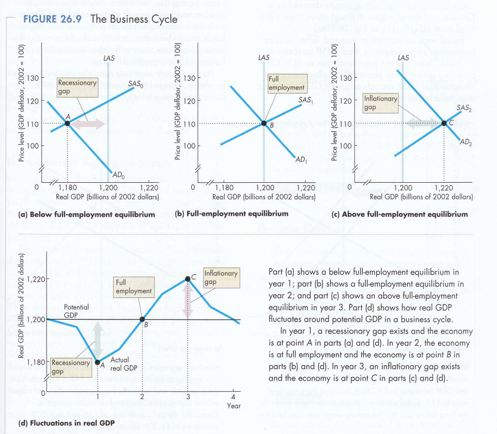
If one moves along the SAS beyond LAS or potential GDP, i.e., after full employment has been achieved, factor prices including the real wage rate will increase due to competition for fully employed factors. That is while in the short run output may exceed potential for example due to overtime and extra shifts it cannot be maintained because competition for fully employed factors of production raises their cost causing production to drop shifting SAS to the left. Thus rather than increased real GDP (which has reached its limit), money factor prices will rise and movement will shift up along the LAS curve reflecting rising final prices for goods and services rather than up SAS (P&B 3rd Ed Fig 24.2). Shifts in SAS occur because of changes in real factor prices thereby affecting a firm’s costs of production. LAS does not shift with changing factor prices because factors or inputs are fully employed. However, changes in the quantity of Capital and/or Labour as well as advances in technology cause shifts in both SAS and LAS (P&B 7th Ed Fig. 26.2; R&L 13th Ed Fig. 23-4). In conclusion, I ask you, after class, as a thought experiment, to consider the impact on SAS and LAS of a change in a national production function and its related factor endowment of Capital, Labour and Natural Resources as well as Technological Change in a field or industry of personal interest and concern. 4.4 AD-AS Equilibrium (MKM C14/339-40: 317-18; 325-327) The purpose of the AD/AS model is to understand and predict changes in real GDP and the price level. It represents another application of the Marshallian scissors of microeconomics. There are both short-run (SR) and long-run (LR) points of equilibrium, that is points to which the model will return after any short-term changes in the underlying variables of the model SR equilibrium occurs when SAD = SAS. If the economy is not in equilibrium forces will tend to bring the economy back into equilibrium (P&B 7th Ed Fig. 26.6; R&L 13th Ed Fig. 23-6). For example, if real GDP is higher than equilibrium, final and factor prices tend to be higher than consumers are willing to pay and firms will cut production, lower prices and factor prices will tend to fall. If, on the other hand, real GDP is less than equilibrium, the quantity of final goods producers supply is less than consumer demand forcing up all prices until equilibrium is achieved. ii - SR Equilibrium & Full Employment (FE) SR equilibrium is not necessarily at potential real GDP or full employment. If it is less there is a recessionary gap; if it is more there is an inflationary gap (P&B 7th Ed Fig. 26.6 & 26.9; R&L 13th Ed Fig. 23-6; MKM Fig. 14.8). Overtime the economy will tend to adjust in response to the forces at play and return the economy to LR equilibrium. For example in a recession, factor prices are depressed causing the cost of production to fall and output to increase over time. During inflation, factor prices are elevated causing the cost of production to rise and output to fall. LR growth shifts LAS to the right, i.e., increased potential. The rate at which LAS shifts is measured by the growth rate of potential GDP. Inflation results when the rate of growth of AD is greater than LAS. As will be seen, a major factor affecting the rate of growth of AD is the quantity of money. If the money supply grows faster then LAS inflation results. If the money supply grows slowly, so does inflation. None of these growth rates are steady but rather there is persistent fluctuation around an ever growing potential GDP. Let us assume that the world economy grows faster than the domestic economy. Demand for exports increases shifting the AD curve (P&B 7th Ed Fig. 26.10; R&L 13th Ed Fig. 23-7 & 24-2 & 24-3).
This shifts the domestic economy out of equilibrium with LAS. Initially movement occurs along the SAS curve on which it is assumed that money factor costs are constant. Eventually, however, factor prices must rise as firms compete for a fixed quantity of factors of production. This raises costs and causes the SAS curve to shift to the left back to LR equilibrium at full employment but at a higher price level. Similarly, let us assume that the price of a significant factor of production like oil increases. This will cause the SAS curve to shift as production costs rise to the left out of equilibrium with potential GDP (P&B 7th Ed. Fig. 26.11; R&L 13th Ed Fig. 23-10 & 24-4). A recessionary gap is created but at a higher level of prices. This combination of recession and inflation is called stagflation. The final outcome depends on what happens to AD. If AD does not increase then the demand for oil is decreased and production falls and other factor prices fall eventually returning the SAS curve to its starting point and the economy returns to LR equilibrium v - Equilibrium Real GDP & Price Level The economy can be in three possible states: a recessionary gap, full employment or an inflationary gap (P&B 7th Ed Fig. 27.10 & 27.11). Automatic forces will tend to eliminate an inflationary gap and restore full employment. There are, however, no automatic forces which will eliminate a recessionary gap. Assume, in the short-run, potential real GDP of $750 billion is greater than actual $600 billion (P&B 7th Ed Fig. 27.10). If autonomous spending increases by $100 billion then AE0 shifts to AE1 and AE increases more than $100 billion due to the multiplier. However, prices increase as AE rises eating into the shift and AE1 drops to AE2. The effect of the price increase is visible in P&B 7th Ed Fig. 27.10; R&L 13th Ed Fig. 23-8. If instead we assume the economy is at long run potential and autonomous expenditure increases AE0 will shift up to AE1 by more than the increase in autonomous spending due to the multiplier (P&B Fig. 25.13). However, because the economy is at full potential this increase in AE will be translated as a shift in AD to the right and in a price increase shifting the SAS to the left (P&B 7th Ed Fig. 27.11). The result is a return to equilibrium potential GDP but at a higher price level. The shifting from below long-run equilibrium to equilibrium and then above characterizes the business cycle (P&B 7th Ed Fig. 26.9:
Non-linked references Jantsch, E. Design for Evolution, Braziller, NY, 1975. White, B. & Hart A-M, (eds), Living Traditions in Art: First International Symposium, Dept. of Education in the Arts, Faculty of Education, McGill University, Montreal, 1990.
|
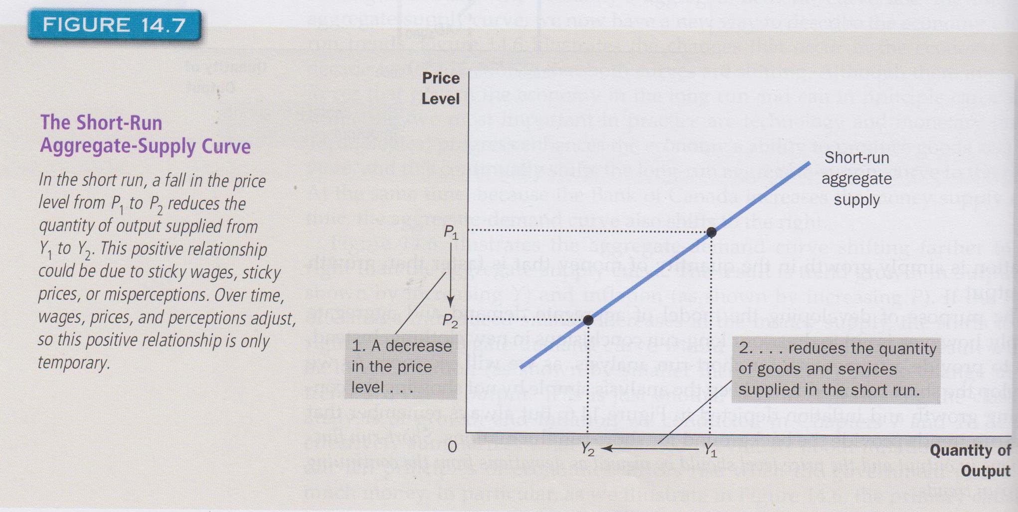 Why? Revenue
goes up (P x Q) while cost (factor prices) remains the same, i.e.,
profits increase. Because real production grows as prices rise SAS
is upward sloping, that is, it has a positive slope. To repeat, higher
prices for goods and services with lower real factor cost in production
increases profits and encourages firms to supply more. Shifts in SAS
can occur due to change in any factor costs and from technological
change (
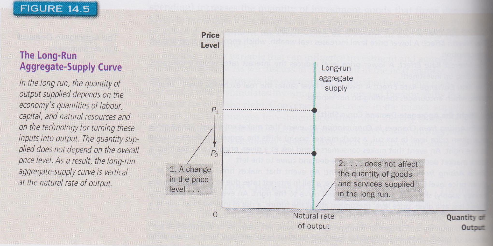 Movement up or down LAS curve is caused by changes in two
sets of prices: (i) the overall or aggregate price level for final goods
and services; and, (ii) factor prices. If final prices go up then factor
prices will rise at the same rate meaning that 'real' wage rates and
other factor prices remain constant as does real GDP.