Mac 2.1

In the Standard Model of Macroeconomics, a national economy is driven by the demand for goods & services. Internally this demand is made by households (consumption and savings), business enterprise or firms (investment) and government (tax & spend) - national, regional & local. Externally, demand is made for domestic goods & services by foreign governments, firms and households in the form of exports.

For the moment we will assume a closed economy, i.e., no imports or exports. This is an autarky, a self-contained, self-reliant national economy in which its citizens can only buy what they make. European colonial empires strove to be autarkies with the colonies providing markets and resources ever increasing the metropole's wealth while constraining potential colonial competition to Imperial home industries and interests. Ideally, they would not have to trade with rival empires for markets or resources. The German Third Reich, the Japanese Co-Prosperity Sphere and then Communist Bloc Nations all aspired to autarky, independent of the market-driven West. They strove to be completely self-contained and self-sufficient. How did that work out?

Each of the three domestic economic actors - households, firms and government - has an objective function, i.e., it strives to maximize some objective, subject to some constraint. In introduction the nature and objective function of each is examined within the framework of the Circular Flow of National Income. Put another way, let's follow the money (MKM Fig. 5.1; MBB Fig. 2.6; R&L Fig. 20.01).

It is assumed that households are the basic unit of consumption and savings. In a household individuals share capital assets like appliances, cars, entertainment centres, housing, etc. It is also assumed that households own all factors of production including capital, labour and natural resources. Households earn income by selling these factors to firms and receive, in return, dividends/interest/profits, wages & salaries and rents. The total income earned by households from the sale of factors of production constitutes Gross Domestic Income (GDI).

In what follows it is assumed that the dollar value of GDI, Consumption (C), Investment (I) and Government (G) spending are expressed in real not nominal terms. As was seen under 2.1 National Accounts, inflation reduces the value of a dollar. This means a dollar in the past bought more than a dollar today or tomorrow. Economists are concerned with what was really bought and sold, e.g., the number of cars, houses, labour, TVs, etc. Inflation adjusting dollars of yesterday yields their real value today. Measuring in a past year's dollars yields their nominal value. As a consequence, inflation eats away at real household income over time.

Some household income is also taxed away by government leaving households with disposable income. Some of this is spent (consumption) and some saved. At the macroeconomic level it is important to note that how much is spent and saved depends on national income Thus consumption and saving are dependent variables induced by changes in national income.

The objective function of households is to maximize their well-being, happiness or, as in microeconomics, their utility. They are constrained, however, by the demand for factors of production, especially labour, and the price of goods & services as well as government policies.

It is assumed that business enterprise or firms are the sole source of goods & services to satisfy the demand of households, other firms and governments. Firms buy factors of production from households. They combine them to produce goods & services. The value of all final goods & services produced by all firms constitutes Gross Domestic Product (GDP). A more detailed explanation of both GDI and GDP is provided in 2.1 National Accounts. As will be seen, GDI ≡ GDP where the symbol (≡) represents an accounting identity meaning that GDI must equal GDP. What is earned by households selling factors of production to firms must, allowing for government taxes and transfers, equal how much households spend buying goods & services from firms.

Assuming households pay all taxes, after paying for factors of production firms use residual revenue to invest in capital plant & equipment to produce the same output or produce more in the next year. Thus investment consists of two parts. The first is depreciation of exiting plant & equipment that wears down and must be renewed to maintain the same output next year. The second part is spent on new plant & equipment to expand production. Thus net new investment is total investment less depreciation. It is important to note that the decision to invest is not dependent on national income but rather on the expectation of profit. Thus investment is an autonomous variable, independent of national income.

The objective function of firms is to maximize profits constrained by the cost of factors of production, available technology and government policies.

It is assumed that governments produce nothing. Thus in Fig 5.1 (above) there is no government. They tax households reducing gross to disposable income. They then redistribute tax revenue to buy both private and public goods & services from firms.

The objective function of government is re-election constrained by satisfaction of a majority of households with how their taxes are spent. It is important to note that government spending is thus autonomous of national income.; it is dependent on political forces. For those interested in such forces, please see Observation #2: The Economics of Democracy.

In what follows it is important to distinguish between planned and actual expenditures by each of the three economic actors. Decisions today about what to buy, or to save, depends on what one expects to happen tomorrow. If one expects prices to fall tomorrow one holds off spending today and vice versa. If one expects to lose one's job tomorrow one reduces spending today and vice versa. If a firm expects demand for its goods & services to increase tomorrow then it invests today and vice versa. If a government expects to be defeated in an upcoming election it spends 'to buy votes' to improve its chances and vice versa. This is Futurity: One lives in the Future but acts in the Present. What happens if one is wrong? What if demand does not increase but one has made an investment to produce more goods & services? To sell the surplus one must lower one's price. There is thus an inherent tension between planned and actual expenditures by one, two or even all three actors. We will later examine how the model adjusts to differences between planned and actual expenditures.

When it comes to spending price plays a critical role. In the Standard Model of Market Economics the determining variable is the market price of a good or service . In macroeconomics, however. it is the overall or Aggregate Price Level of millions of different goods & services. The Aggregate Price Level is measured by a 'price index' of all goods & services. This is possible because, as will be seen in 5.2 Monetary Policy, money serves as a unit of account for apples and oranges and all other goods & services.

Given the critical role of price we begin to construct the Standard Model of Macroeconomics with the assumption that all economic actors - households, firms and governments - share the same expectations about the Aggregate Price Level. For a given price level each plans its expenditures. Change the price level and spending changes. We assume, for the moment, that the Aggregate Price Level is, in effect, fixed. What this means is that an increase in demand will not result in an increase in the aggregate price level. This was the situation when Keynes wrote his General Theory in 1936 in the depths of the Great Depression. There were so many unemployed resources - capital, labour, natural resources, etc.. - that an increase in demand would have no effect on the aggregate price level.

Taken together, spending by households (C), firms (I) and governments (G) constitutes Aggregate Expenditure or:

I = Investment by firms in plant, equipment and inventories including residential housing;

GDI = gross domestic income earned by domestic factors of production including capital, labour and natural resources; and,

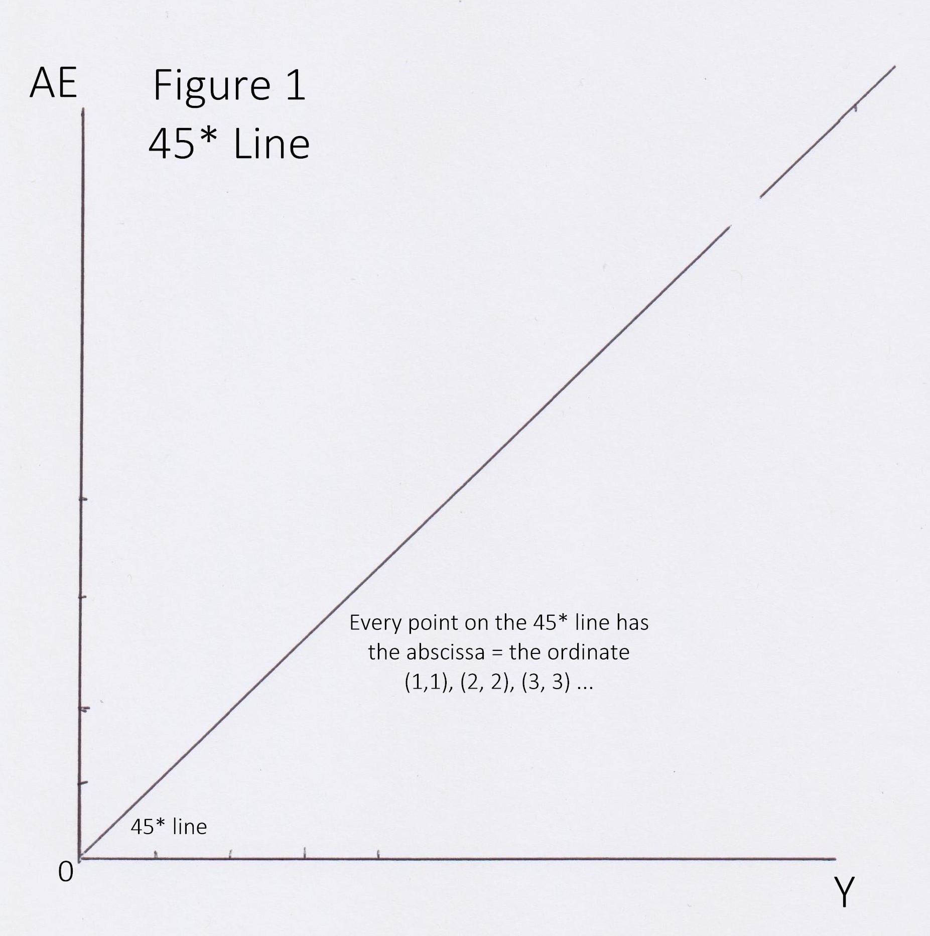
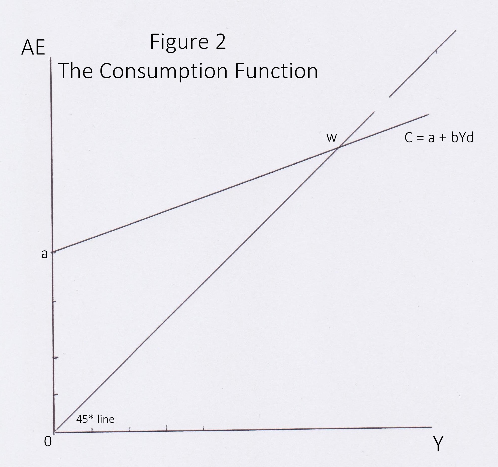
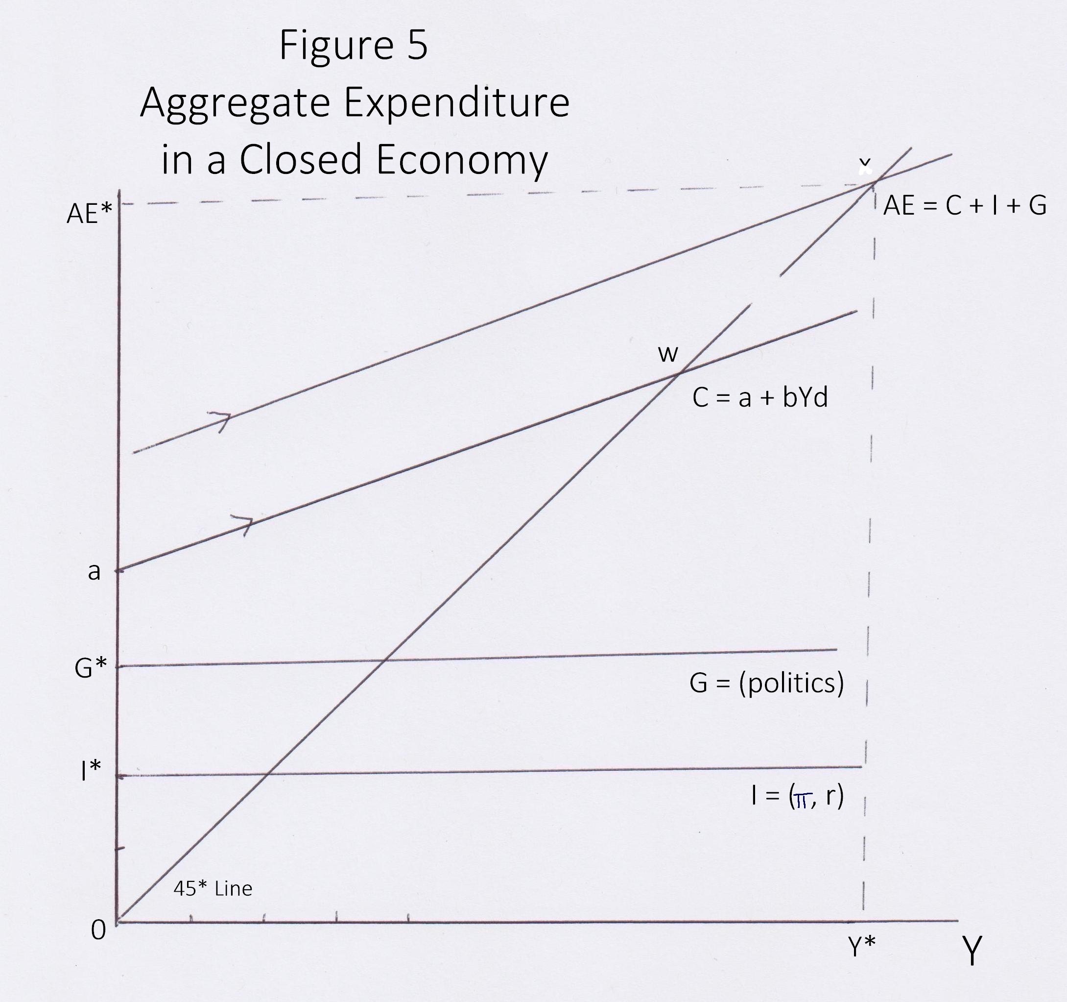
In this section we examine each component of AE. We begin in a closed economy with the Aggregate Price Level (P) fixed and equilibrium existing where AE = Y. Graphically this is represented by a locus of points forming a 45 degree line drawn from the origin of Y represented as the X-axis and AE by the Y-axis. AE = Y at every point on the 45 degree line (Fig. 1).

Consumption (C) is the final use of goods and services by households to satisfy human wants, needs and desires. Savings (S) is the difference between income and consumption. In a sense savings is deferred consumption.

The primary factor affecting consumption and savings is disposable income (Yd) which equals gross household income less taxes plus government transfers. This means that changes in taxes to and transfers from governments such as unemployment insurance, welfare, etc., changes Yd. As disposable income increases, consumption and savings increase and vice versa. Thus C & S are induced by changes in Yd

The relationship between disposable income and consumer spending is the Consumption Function (Fig. 2). If we plot income (Y) on the x-axis and consumption (C) on the y-axis then point 'w' on the 45 degree line shows where consumption equals disposable income (P&B 7th Ed. Fig. 27.1; R&L 13th Ed Fig. 21-2). The Consumption Function is expressed as:

Yd = disposable income, i.e., gross income minus net taxes (taxes minus transfers).

Non-discretionary or autonomous consumption (a) varies between countries and over time. Thus in Saskatoon winter heating is essentially non-discretionary for survival. In Trinidad there is no need for winter heating. Similarly, once upon a time a telephone was a luxury and 'party lines' common. Today a smart phone is a near necessity.

In the figure the area between the Consumption Function and the 45 degree line ending at point 'w' consumption is greater than income. To support consumption households must 'dis-save', i.e., sell off assets accumulated in the past or rely upon charity, family, friends or government transfers. After point 'w' disposable income is greater than consumption. This means households are able to save part of their disposable income. Such savings then become available for investment purposes.

The marginal propensity to consume (MPC or b in the figure above) is the slope of the Consumption Function. It measures how much of each additional dollar in income is spent on consumption (P&B 7th Ed Fig. 27.2; R&L 13th Ed Fig. 21-2). The MPC also varies between countries and over time. For example, the MPC is much higher in North America and western Europe than in East Asia. This means there is a higher level of savings in East Asia. Similarly, before the Great (sometimes called 'the Long') Recession of 2008 the MPC in the United States was arguably greater than 1. This meant households spent more than they earned. Essentially they borrowed from East Asian savers. After the Great Recession the MPC has fallen below 1 as Americans pay off their debts.

One factor affecting MPC is progressive income tax - the higher the income, the higher the rate of taxation. The percentage of each additional dollar of income taken by government is the marginal tax rate (MTR). Under progressive income tax the MRT rises with income. Accordingly the Consumption Function bends lower as it passes from a lower to a higher MTR. Thus, in effect, the MPC changes as disposable income is reduced by a higher MTR. Therefore, under progressive taxation, the slope of the Consumption Function becomes MPC minus a changing MTR. In effect, taxes are a leakage from the system reducing the consumption of households.

Savings (S) is the difference between disposable income (Yd) minus consumption (C). In the figure above dis-saving occurs from point 'a' to point 'w'. At point 'w' savings are zero. Above point 'w' disposable income is greater than consumption and savings occur. Given that disposable income is split between consumption and savings the Marginal Propensity to Save (MPS) is (1-b) where 'b' is the MPC (P&B 7th Ed Fig. 27.2; R&L 13th Ed Fig. 21-3). Other influences on savings include changes in: the interest rates (r); the value of net assets, i.e., changes in the aggregate price level (P); and, expected future income. 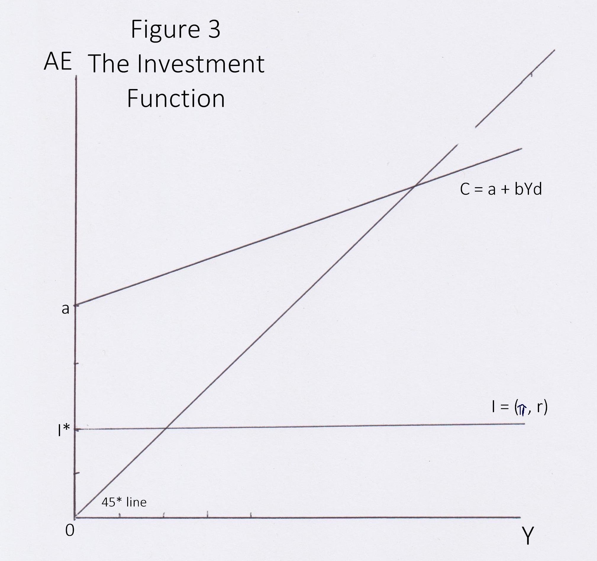Such changes shift the consumption and savings functions.

Each firm has a list of investment projects that can be rank ordered according to their expected rate of return or profit (π). Their ordering is then compared to the opportunity cost of money, i.e., the interest rate (r), i.e., what could be earned using the same money to buy a financial asset with a guaranteed rate of return. Below is an example of the 'marginal efficiency of capital schedule' introduced by Keynes.

In the example Projects 1-4 are all expected to earn a higher profit than the current 9% interest rate. They are undertaken. Project 5 promises a profit rate equal to the interest rate but with risks. A bond will return a fixed interest rate but an investment has risks (economic, legal or political). Why take the chance? Projects 5-10 will not be undertaken.

What happens, however, if the interest rate drops to 5%? Projects 5-8 are now profitable. What happens if the interest rate goes up to 10%? Then only Projects 1-3 will be undertaken. What is important is that if the interest rate falls then investment increases and vice versa. As will be seen in 5.2 Monetary Policy it is by raising and lowering the interest rate that the central bank can reduce or increase investment and thereby affect GDP.

Investment is some function of the expected rate of return or profit (π) and the interest rate (r), or

In this sense, investment is autonomous to Y. Being autonomous firms independently determine which projects to undertake, i.e., how much to invest, without regard to Y. The Investment Function is a straight line with a slope of 0 beginning at I₁(Fig. 3).

While mainstream economists stress rationality in calculating the Marginal Efficiency of Capital Schedule, Keynes stressed its limits in Chapter 12: The State of Long-Run Expectations of his 1936 The General Theory of Employment, Interest and Money. Among other things he noted three things.

First, there are two types of investment. The first is to build an Enterprise (investing for the long-run); the second is Speculation (playing the market). For Keynes the stock market was a 'beauty contests' in which one tries to anticipate what the crowd will considers the best looking investment tomorrow. Similarly, at the beginning of the Great Recession of 2008 another meme emerged - 'the roulette economy'.

Second, there is simply ignorance, not just uncertainty about the future. With an investment spreading over many years, e.g., a dam, power station, integrated chip factory, it is simply impossible to know what the price of copper may be in 10 years time let alone the overall state of the economy. Probabilistic estimates can be made for uncertainty but not for ignorance, the lack of knowledge.

Third, Keynes believed that investment involved the 'animal spirits' of the entrepreneur. He summed it up this way:

It is safe to say that enterprise which depends on hopes stretching into the future benefits the community as a whole. But individual initiative will only be adequate when reasonable calculation is supplemented and supported by animal spirits, so that the thought of ultimate loss which often overtakes pioneers, as experience undoubtedly tells us and them, is put aside as a healthy man puts aside the expectation of death (Keynes, 1936, 162).

There is a cycle to such 'animal spirits' fuelled by greed as the market soars and fear when it dives. They are bi-polar. According to Keynes, this is what fuels the business cycle. Years later another economist summed it up this way:

Keynes’s whole theory of unemployment is ultimately the simple statement that rational expectation being unattainable, we substitute for it first one and then another kind of irrational expectation: and the shift from one arbitrary basis to another gives us from time to time a moment of truth, when our artificial confidence is for the time being dissolved, and we, as business men are afraid to invest, and so fail to provide enough demand to match our society’s desire to produce. Keynes in the General Theory attempted a rational theory of a field of conduct which by the nature of its terms could be only semi-rational. But sober economists gravely upholding a faith in the calculability of human affairs could not bring themselves to acknowledge that this could be his purpose.

Shackle, G.L.S., The Years of High Theory: Invention and Tradition in Economic Thought 1926-1939,

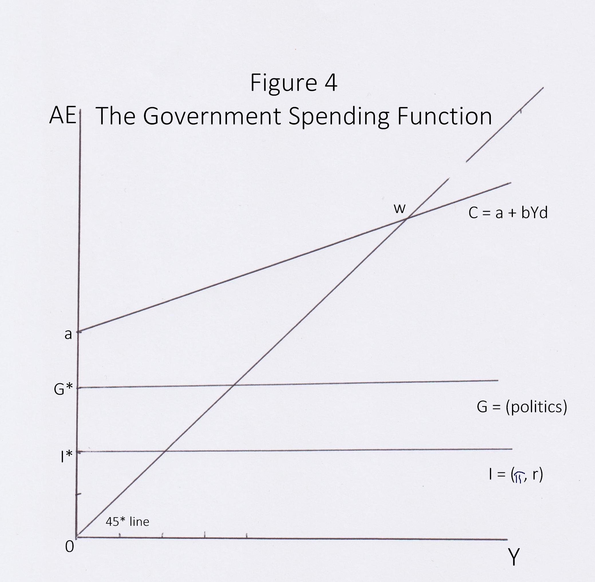
Government spending is funded by taxes on household income and/or borrowing on financial markets. It is determined politically, that is government spending influences Y but Y does not influence government spending. Government spending is a political, not an economic decision. In this sense, government expenditure is autonomous of real GDP. The Government spending Function is expressed as:

For those interested in the nature of such decisions, please see Observation #2: The Economics of Democracy. The Government Spending Function is a straight line with a slope of 0 beginning at G₁(Fig. 4).

To plot the AE curve we must add, vertically, C + I + G at each level of Y. Given that the slope of I & G is zero the slope of the final AE curve as shown in the figure below is the same as the Consumption Function (b) or the marginal propensity to consume (MPC).

It is important to note that AE is determined by first assuming that: the Aggregate Price Level (P) is fixed; it is a closed economy meaning there are no imports or exports; and the Marginal Tax Rate (MTR) is constant or 'flat'. The economy is in a state of autarky, self-sufficiency. Equilibrium occurs at point 'v' (Fig. 5).

Actual aggregate expenditure is always equal to real GDP. Planned and actual aggregate expenditures or real GDP, however, can diverge. How? It is assumed that C, G, X & M planned expenditures will be fulfilled. That leaves Investment (I) as the component that may vary. This is due to inventories. When aggregate planned expenditure is less than actual, inventories increase; if actual is greater than planned, inventories shrink. This sets up a dynamic in the next time period. Keynes's introduction of inventory adjustment suggested recessions or downturns in the economy averaging about half a year. Once inventories are run down, production starts up again. Thus, one the one hand, while some output may not be sold, factors of production were employed and income earned by households during this time period contributing to GDI. On the other hand, the excess or inventory will be sold off in the next time period but no new factors of production will be employed, no new income earned and hence no increase in GDI during that time period.

We now change our assumption and open the economy to world trade. Why we should do so is explained in 6.0 The Global Economy.

Exports are goods and services sold to persons (Legal or Natural) of another country plus services involved in shipping, financing and facilitating exports. Their level is determined by international price (exchange rate) of the $Cdn, the real GDP of foreign countries (GDP_f) and trade agreements.

All things being equal: the lower the Canadian dollar, the higher the real GDP of foreign countries and the more liberal trading agreements and the higher will be exports. The Export Function is expressed as:

Exports are autonomous of Y. The Export Function is a straight line with a slope of 0 beginning at X₀ (Fig. 6).

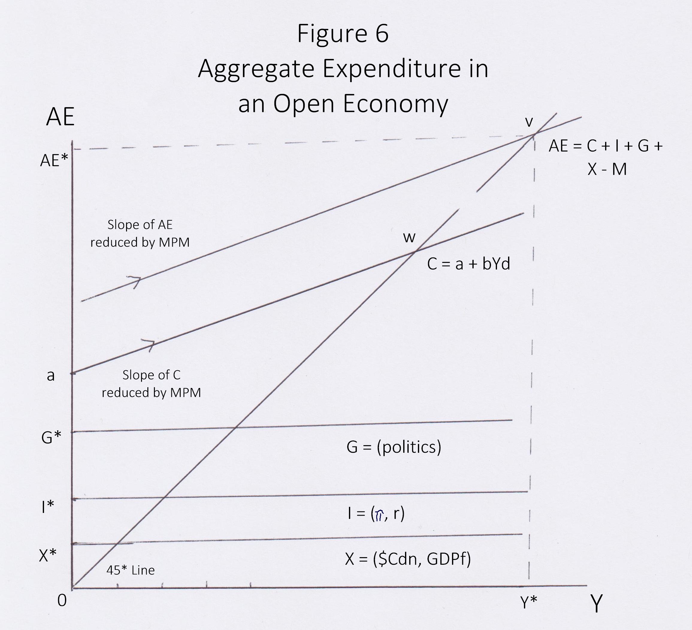
Imports are goods and services bought by Canadians (Legal or Natural) from another country plus services involved in shipping, financing and facilitating exports. Their level is induced by Canadian real GDP (Y) and affected by the exchange rate for the $Cdn and trading agreements.

The Import Function is the relationship between Y and imports, assuming all other factors are held constant. Imports are induced by changes in Y. The Marginal Propensity to Import (MPM) measures the change in imports divided by the change in Y, i.e., MPM = change in imports/change in income (P&B 7th Ed Fig. 27.3; R&L 13th Ed Fig. 21-6). Accordingly, of every additional dollar in disposable income some is saved (MPS) but the rest is spent consuming both domestic and imported goods & services. This means that the slope of the Consumption Function and hence the AE curve will be reduced depending on the value of MPM.

Net exports is equal to actual exports minus imports (R&L 13th Ed Fig. 22-1 & 2 ).