Microeconomics
Macroeconomics
SISTERetrics
SITES
Compleat World Copyright Website
World Cultural Intelligence Network
Dr. Harry Hillman Chartrand, PhD
Cultural Economist & Publisher
©
h.h.chartrand@compilerpress.ca
215 Lake Crescent
Saskatoon, Saskatchewan
Canada,
S7H 3A1
Launched 1998
|
Microeconomics 5.0 Competition
|
|
|
Perfect Competition (MKM C4/68-9; 63-4, 65-66; 59-60) fully satisfies the following four strict conditions:
i -
Anonymity
ii - No Market Power
iii - Perfect Knowledge
iv - Free Entry & Exit
(MKM
C14/304-7; 286-87;
310-311;
289-291)
2. Profit Maximizing Output
If
these strict assumptions are satisfied then there is a perfectly
competitive marketplace and the firm is a 'price
taker'. The market sets the price. If a firm raises its price above
market price it loses all its business because of homogenous goods and the perfect knowledge of buyers.
Why pay a higher price for an identical product? If a firm
lowers its price below market it will, as will be seen,
sell less at a lower price earning smaller revenue and profit. To determine
profit-maximizing output we can use
two methods:
i -
total revenue
(TR) less total cost (TC); and,
ii - marginal analysis.
i -
Total Revenue less Total
Cost
Profit
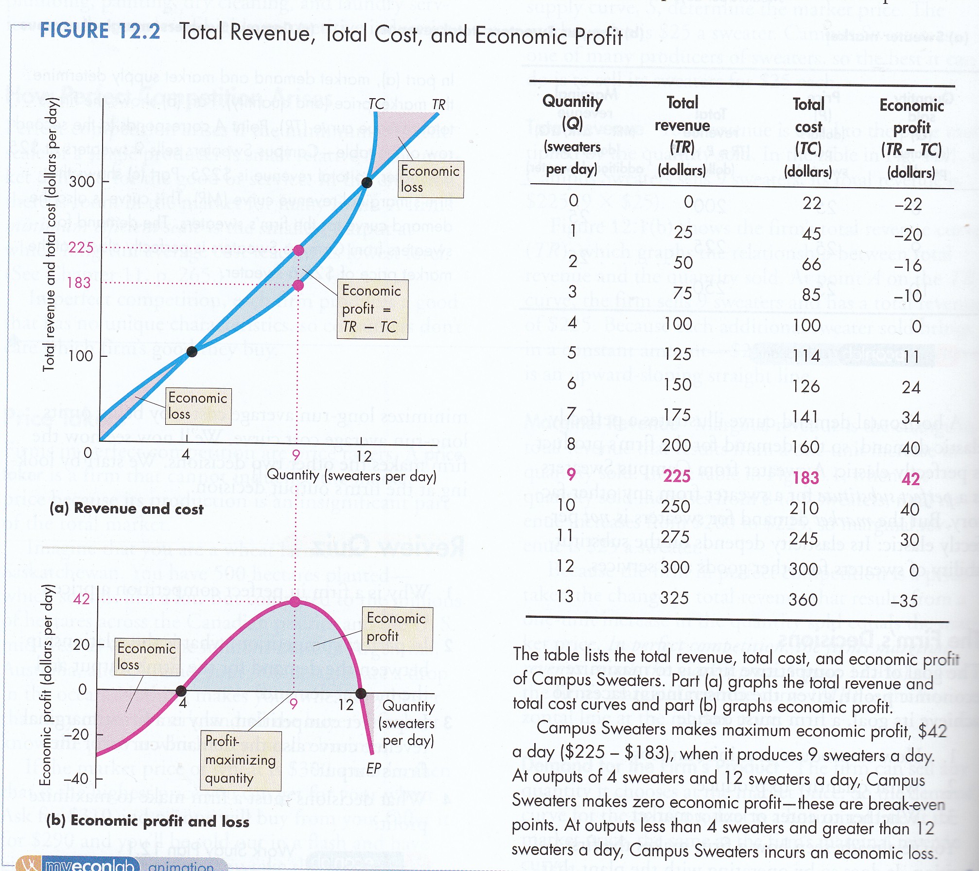
(π) equals total revenue (TR) minus
total cost (TC). Under
perfect competition a firm sells every unit at market price. It is
a price taker. In Cartesian space (Quantity, Price/Cost) the TR
curve is a straight 45º line radiating from
the origin (0, 0). reflecting the fact that each unit sold earns the
same revenue. The TC curve, on
the other hand, begins above the origin on the y-axis reflecting fixed
costs that must be paid even if no revenue is earned. The changing
distance between TR and TC shows economic loss or profit (TR - TC
< 0 or > 0). Initially there is economic loss followed by profit followed by
loss with two points of ‘normal’ profit where TR - TC = 0 (P&B
7th Ed Fig. 12.2; R&L 13th Ed
Fig. 9-4i).
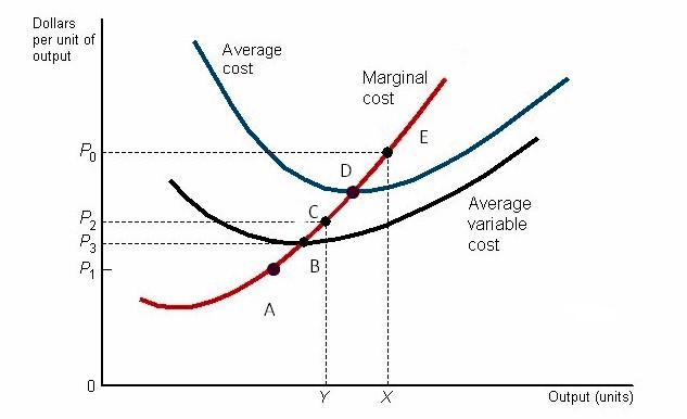
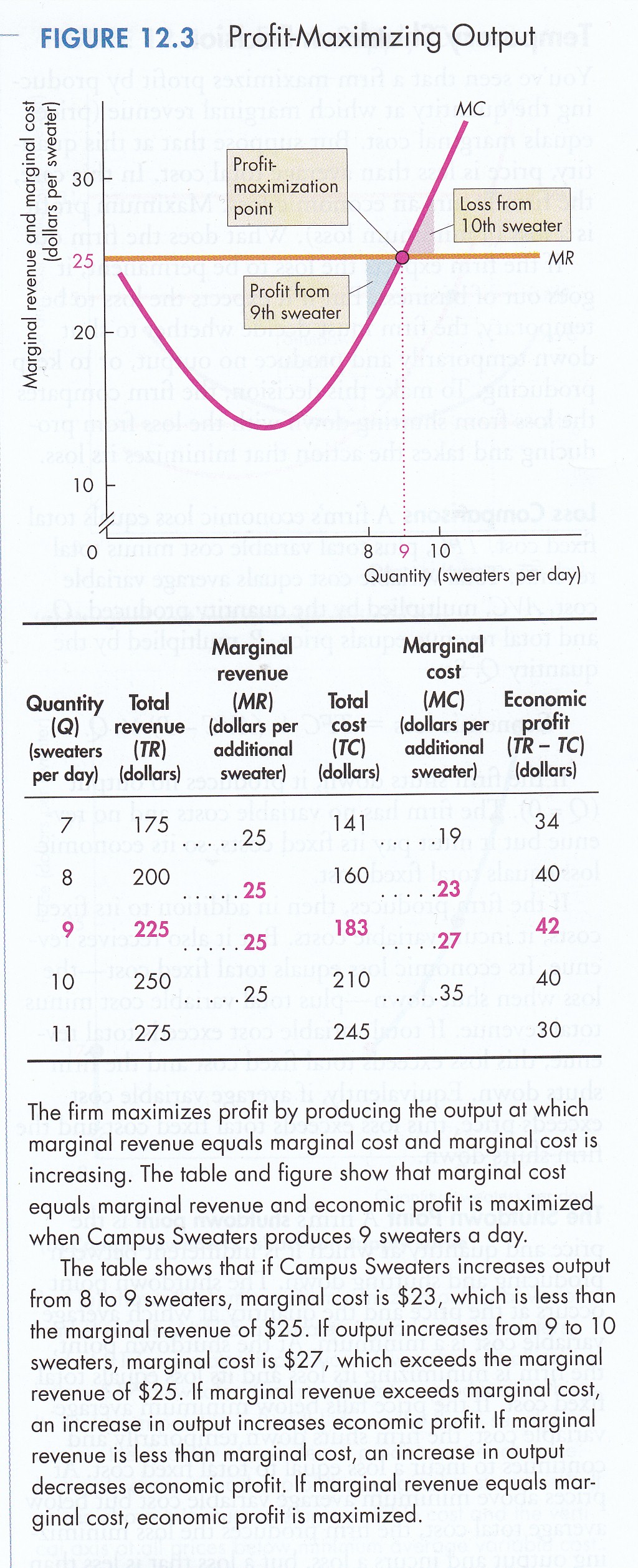
ii - Marginal Analysis Given an upward sloping marginal cost curve, profit maximization occurs (under all forms of competition) where the revenue earned on the last unit sold (marginal revenue) equals the cost of the last unit sold (marginal cost), i.e., where MR = MC. Under perfect competition, however, MR equals P (each unit sold at market price) and profit maximization is where MR equals P equals MC. If MR is greater than MC then producing an additional unit adds more revenue than cost. If MR equals MC then the firm experiences normal profit with all factors of production including entrepreneurship earning their opportunity cost. If MR is less than MC then producing and selling another unit results in a loss. In effect the firm faces a perfectly horizontal or elastic demand curve fixed by market price (P&B 7th Ed Fig. 12.3; R&L 13th Ed Fig. 9-4ii; MKM C14/Fig. 14.1). An upward sloping marginal cost curve also explains why a perfectly competitive firm will not lower its price below market price. If MR falls profit maximization still occurs where MR equals MC and we slide down the MC curve to equilibrium a smaller output, lower total revenue and less profit. Why lower one's price if one earns a higher profit by taking market price? It is more thus profitable to be a 'price taker'.
3.
SR Equilibrium
There are five
i - point A shows a
ii - point B is the shut down point. The firm earns enough to pay its variable costs but none of its fixed costs. It opportunity cost is the same: if it stays it must pay fixed costs out of pocket; if it exits it must pay fixed costs out of pocket. This the starting point of the firm's supply curve. It will not produce unless it receives at least P3; iii - point C shows a loss with market price between shutdown (B) and break even (D). In this case the firm earns enough to pay all variable and some fixed costs. It minimizes losses by staying in business in the short run. If it exits it must pay all fixed costs without any revenue. In the long run, however, the firm must decide if the exit of loss making firms in (i) will raise market price to achieve normal profit or if economies of scale are available to reduce marginal cost so that normal profit can be earned in the long run;
iv -
v -
4.
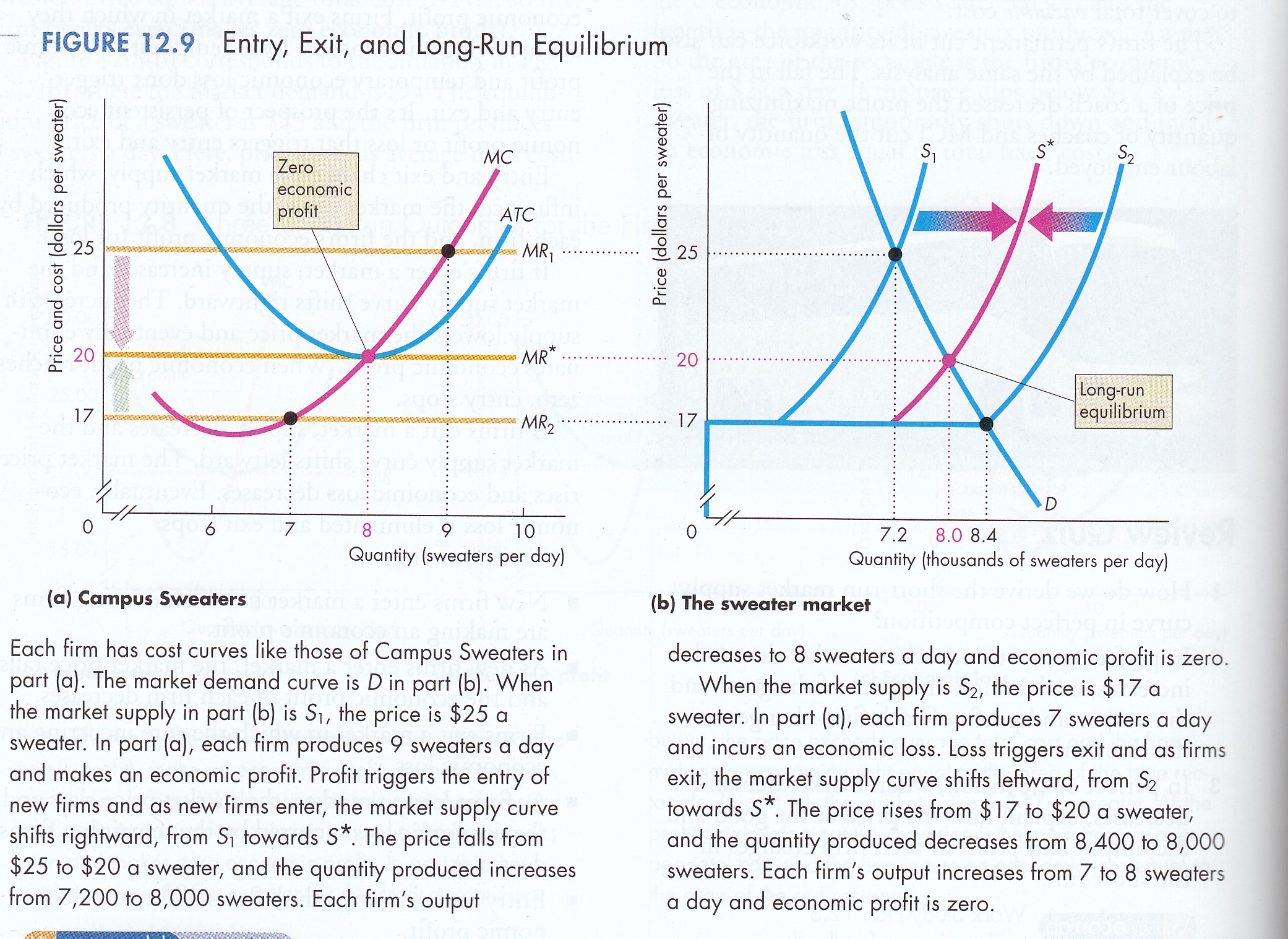
LR Equilibrium
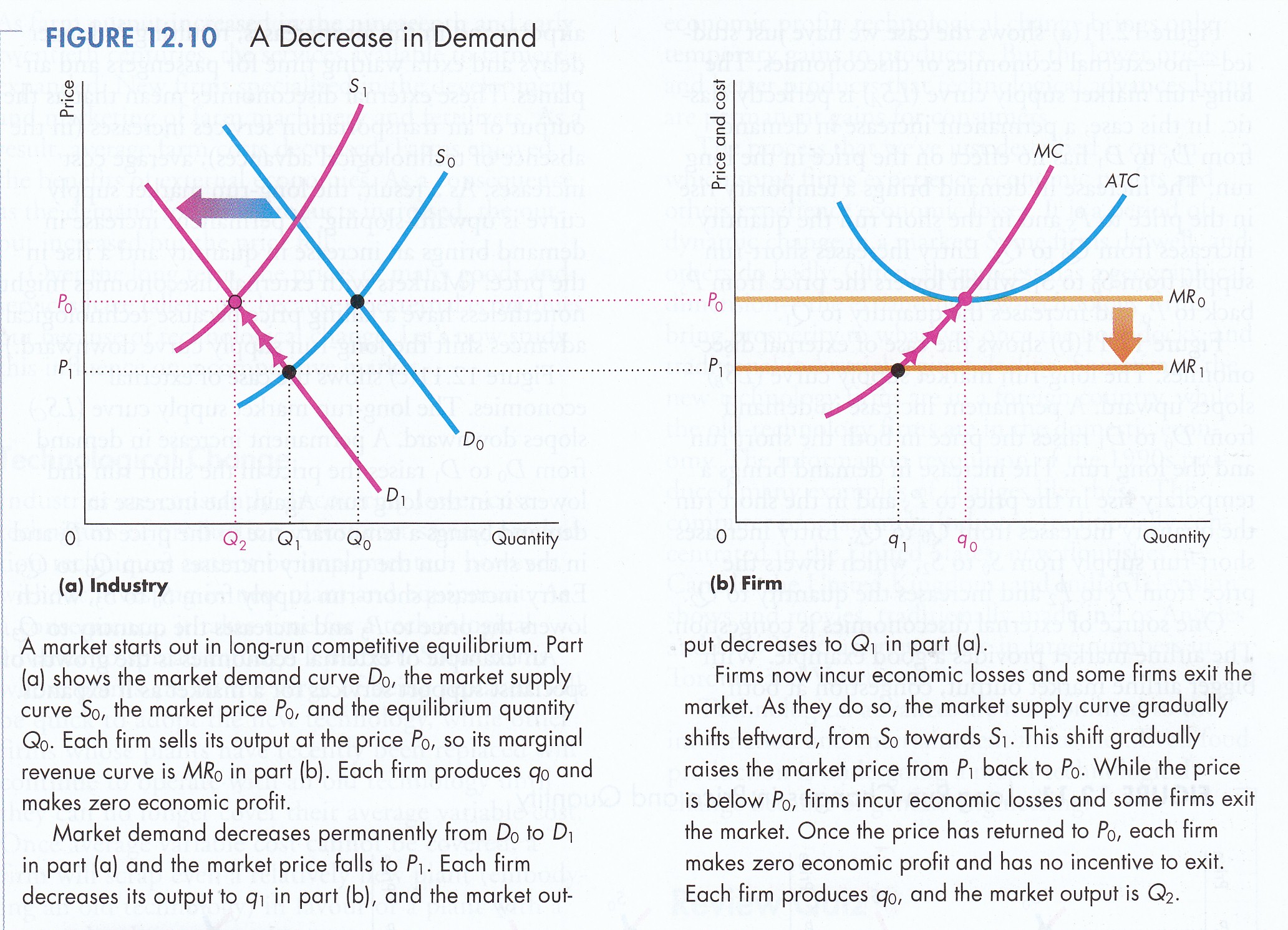
In the long run firms suffering losses with market price below shut down exit the industry shifting the market supply curve to the left raising market price. Similarly, firms that suffer losses with market price between shut down and break even and that do not expect market price to rise sufficiently due to the exit of other loss making firms or cannot benefit from economies of scale also exit. This process will continue until all loss making firms exit and market price reaches break even for all remaining firms.
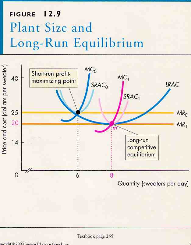
Assuming
economies of scale in the
long-run, firms suffering losses with market price between shut sown and
break even adjust the size of plant creating a series of
short-run average and marginal cost curves. The long-run average
cost curve is an envelope of short-run average cost curves.
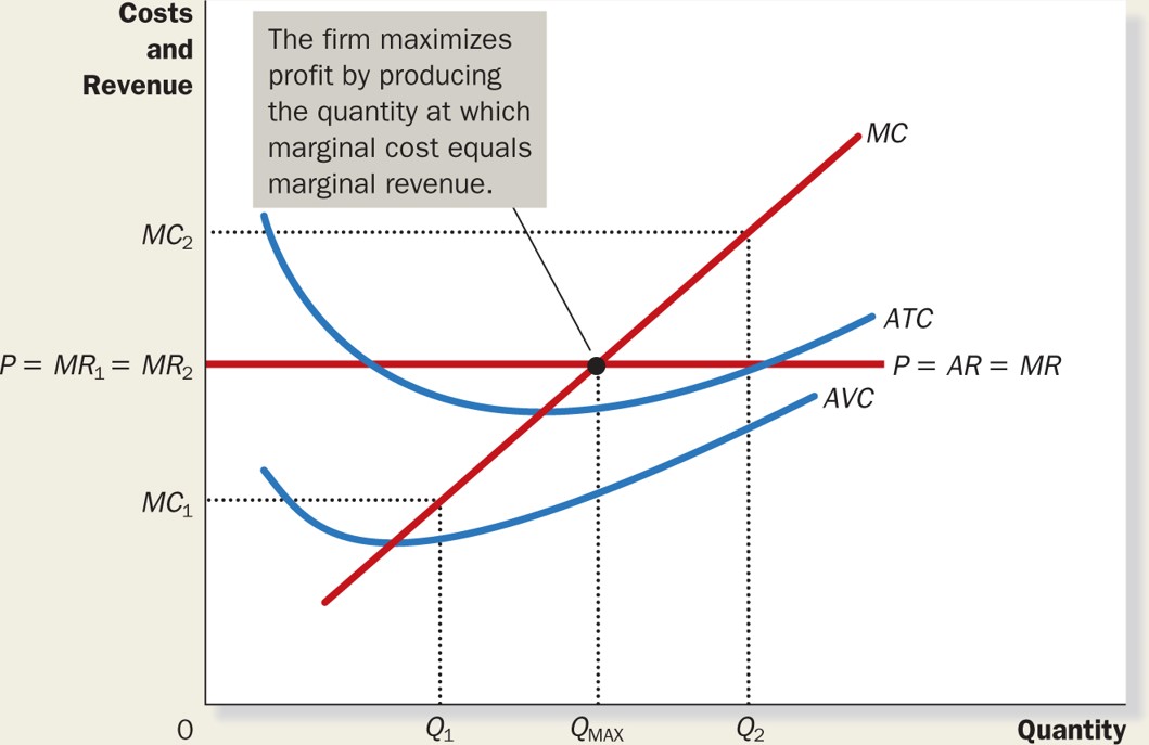
If economic profit is being earned in the long run new entrants shift the supply curve to the right lowering market price. Entry will continue until market price eliminates excess profits and reaches break even for all remaining firms. But what of the demand curve faced by the perfectly competitive firm? Market price rules as the demand curve. If Firm A raises its price above market - given homogenous goods and perfect knowledge - consumers will not buy from Firm A but rather from other firms at market price. What if Firm A lowers its price below market? Given profit maximization occurs where MC = MR and MC is upward sloping (P&B 7th Ed Fig. 12.3) the reduction in price (MR) means output decreases. Firm A is left with lower sales (total revenue) and lower profit than if it simply accepted market price. Hence we call a perfectly competitive firm a 'price taker' in that to maximize profit it must accept market price. The perfectly competitive firm does not face the market demand curve but rather market price like a perfectly horizontal demand curve.
5.
External Economies, Changing Taste & Technology
To this point it
has been assumed that cost is a function only of firm output but cost may
depend upon the output of all firms in the industry.
For example, if industry output goes up, input costs to the firm
may go down, i.e. an external economy to the firm’s production.
Or, if industry quantity goes up, factor costs to the firm may
increase, i.e., an external diseconomy to an individual firm’s production.
There are also what can be called enabling or transformative innovations
outside the economy itself in the form of scientific breakthroughs or
within the economy through the spreading of new techniques such as
'just-in-time' inventory systems or communications innovations such as
the internet or
QR Codes.
Furthermore, such external effects may be ambiguous, that is they
may increase the cost of some and decrease the cost to other firms.
Firms base their behavior on their own marginal cost curve. If all anticipate the same market equilibrium price and industry output is consistent with the summation of individual firm output there will be no further adjustment. Otherwise, individual firm output may not equate with marginal cost and it will adjust in the next round of what is called tatonnement or a bidding process until there is no further adjustment. The market supply curve should state optimal output as a function of price after all necessary adjustments.
In
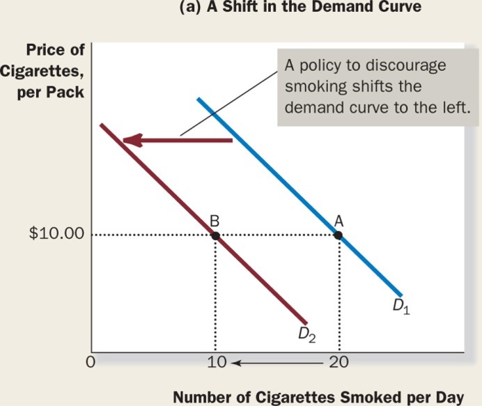
addition to external economies, changes in taste and production technology
itself can change
equilibrium. Taste is symbolized by
the f in preference function U = f (x, y) while technology
is symbolized by the g of the production function Q = g
(K, L). A decline in
taste for a commodity can permanently reduce demand (shift curve to left)
lowering price. At the
extreme, all firms exit and the industry collapses (hoola-hoops) (
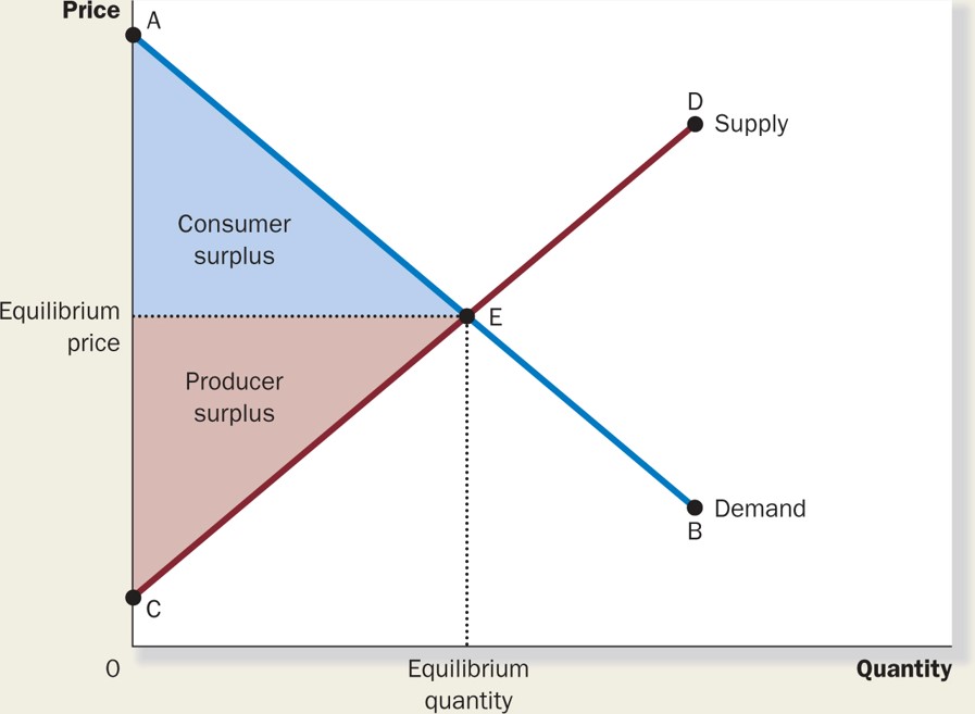
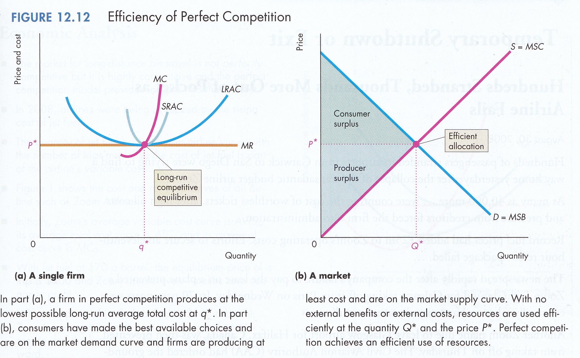
6. Allocative Efficiency
Allocative
efficiency implies all factors of production and all commodities demanded
by consumers are in their best use and receive their opportunity cost. Further, it is assumed that there are no external cost or
benefits, i.e. all external costs and benefits have been ‘internalized’.
Three conditions must hold:
i - Consumer Efficiency:
when consumer cannot increase utility by reallocating budget:
ii - Producer Efficiency: when firm cannot reduce cost by
shifting input mix:
MPK/PK = MPL/PL
Epithet There are four classes of idols which beset men’s minds. To these for distinction’s sake I have assigned names—calling the first class Idols of the Tribe; the second, Idols of the Cave; the third, Idols of the Market-Place; the fourth, Idols of the Theatre. Francis Bacon (1560–1626), Novum Organum, Aphorism 39 (1620).
Beginning with Thomas Aquinas through Adam Smith up to today when consumers are outraged about bank profits and ‘bitch’ at the gas pump, the ‘just price’ has engaged the hearts and minds of economic thinkers for almost a thousand years in the West. Various theories have been suggested to explain the 'value' of a good or service. These include: (i) scarcity; (ii) utility (as usefulness); (iii) input cost especially the labour theory of value shared by all classical economists including Marx; and, (iv) whatever the market will bear. In this sense, there is a distinction in economics between 'value theory' and 'price theory'. Please see my "Value without Price".
Perfect
competition is the most comprehensive statement of conditions under which such
‘a just price’ exists because it combines all of them in a deductively
logical and mathematically and geometrically demonstrable model.
It generates Bentham's greatest good for the greatest number. Unlike other social sciences in economics 'seeing is believing'.
It is a yantra
Deviations in the
‘real world’ from Perfect Competition is used to justify public intervention.
For example, cases of 'market failure or the failure to achieve the
above requirements of Perfect Competition, justify in the Standard Model
public intervention in the market in order to:
The price/output outcome of perfect competition provides the benchmark against which performance of all other market structures are judged. There is, however, serious questioning about both the pedagogic as well as policy use and application of this benchmark. The last ideology standing after the end of the Market/Marx Wars - perfect competition - serves as the regulatory foundation of the EU, NAFTA, WTO and other multilateral economic trade agreements. It is also why economist Kenneth Boulding rightly notes that economics is a 'moral' not a natural science.
|
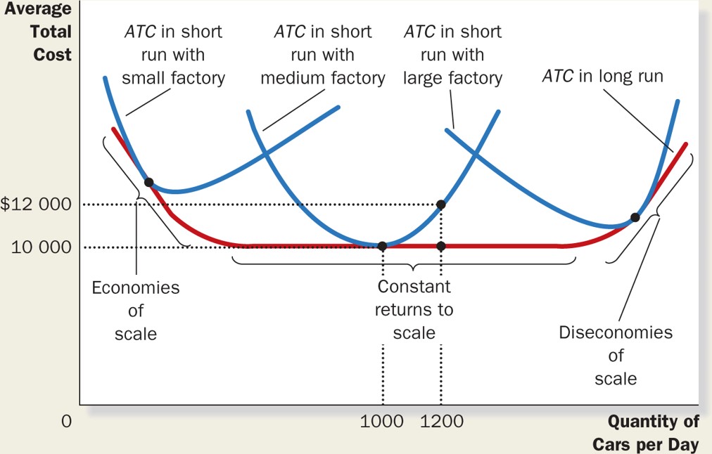 At this size the short-run
marginal cost curves becomes the long-run marginal cost curve
(
At this size the short-run
marginal cost curves becomes the long-run marginal cost curve
(