3.0 Model

3.3 The Monetarist Model (cont'd)

(a) Quick Review
 

3.3.1 Quick Review

a)  Classical

The starting point is the ‘equation of exchange’.  At any given time there are a certain number (or volume) of transactions (i.e. T = the number of buy/sells) in the economy.  The rate at which the same bills ‘turnover’, that is the number of transactions financed with the same bills, is called the velocity of money (V).   There is also a price index (P) for the huge range of goods and services bought and sold.  This is summed up in the equation of exchange (EE) as:

Eq. 4.1              MV  P_TT or,

- the quantity of money times its velocity is identical to the price (level) times the volume of transactions.

This presentation of EE (Eq. 4.1) is an identity in that V is derived as a residual, i.e.,

            Eq. 4.2              V_T 

In this version, however, transactions include not only newly produced goods and services but also second-hand ones.   For only new goods and services corresponding to factor income the EE is:

Eq 4.3               MV  PY where Y is current output and P is the price index.

Again EE is an identity if V is calculated as a residual, i.e.,

            Eq. 4.4              V

In the Classical (and Keynesian) Model, V is determined exogenously by payment habits and payment technology. If so then EE ceases to be an identity.  With Y fixed in the short run by supply-factors and V fixed by institutional factors, EE becomes:

            Eq. 4.5               or

            Eq. 4.6       

An alternative interpretation was offered by the Cambridge School known as the Cambridge approach or the Cambridge cash-balance approach.  This approach stressed that people held money (cash balance) for convenience, compared to other stores of value, in conducting transactions.  However holding cash means that no interest will be earned from investing in productive activities.  Accordingly, how much cash would people hold?  In essence the demand for money was a function of their income, i.e.,

            Eq. 4.7              M^d = kPY where

                        - M^d = the demand for money;

                        - k = a proportion of nominal income;

                        - P = the price level; and,

                        - Y = real income.

Given, according to the Cambridge approach, that cash was desired due to its usefulness in transactions and that the volume of transactions was a function of income then the demand for money varies according to level of income.

In equilibrium, the supply of money (exogenously determined by monetary authorities) would equal the demand for money, or,

            Eq. 4.8              M = M^d = kPY where,

                        - k is assumed fixed in the short run; and,

                        - Y is determined, as before, by supply factors.

The Fisher version (Eq 4.5) and the Cambridge approach (Eq. 4.7) become roughly the same if V = 1/k.  Thus if people hold 1/4th of their nominal income as cash then the number of times the average dollar is used equals four. 

The big change with the Cambridge approach is the formal introduction of the demand for money.  It also allows an assessment of the impact of the quantity of money on the price level (Fig. 4.1).  If the quantity of money increases but output is fixed then people will use the extra cash to consume or invest.  Increased demand for goods raises their prices: too much money chasing too few goods.  If Y is fixed as assumed in the Classical model and k is constant then a new equilibrium will be established at which the increase in money leads to a proportionate increase in price – same output, higher prices, i.e. inflation. 

b) Keynesian

Total demand for money in the Keynesian Model or MD = TD + PD + SD where TD and PD vary positively with income and negatively with respect to interest rate while SD does not vary with income but negatively with respect to interest rates.  Taken together we can say:

(6.3)          Md = L(Y, r)

and if we assume the function is linear then

(6.4)          Md = co + c1Y – c2r where c1 >0, c2 >0 where:

c0 is the minimum amount of cash that must be held;

c1 is the increase in money demanded per unit increase in income; and,

c2 is the decrease in money demanded per unit increase in the interest rate. 

Firms borrow money from households to finance investment projects by issuing bonds (a proxy for all interest generating assets).  The price they pay for this money is the interest rate.  As previously noted Keynes assumed firms had an investment schedule that measured the expected profit rate to be earned from alternative projects mapped against the rate of interest.  If the expected profit less the cost of money was positive, a firm ceterus paribus will undertake the project; if negative, then the project would not be undertaken.  This is called the 'real rate of return'.

If the interest rate rises, then business borrowing declines; if interest falls, borrowing increases (Fig. 6.1).  If investment increases then aggregate expenditure shifts up by the autonomous increase in I.  This increase through the aggregate expenditure multiplier will lead to an even larger increase in income.   Accordingly, the interest sensitivity of aggregate demand is important in determining appropriate monetary polices.

            In effect the interest rate is determined in two distinct markets.  The first is the market for bonds.  The second is the market for money itself. Therefore one hold one’s wealth (Wh = assets) as either money or bonds (interest generating assets), i.e.,

(6.1)          Wh = M + B

This means that there are two distinct money markets: one for money itself and the other for investment financing.  In the Keynesian Model overall equilibrium is established by the interaction of these two money markets.

i – LM Curve

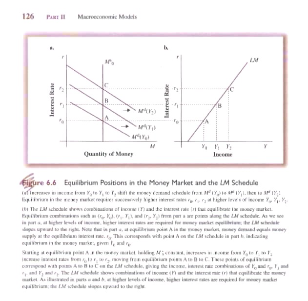
The first is defined by the LM curve (demand for liquidity).  Fig. 6.6 demonstrates equilibrium in the money market given Ms0 and different levels of Y(0, 1, 2).  At Y0 equilibrium is achieved at r0.  If Y increases to Y1 then transactional demand increases but with a fixed money supply this increased demand raises the price of money, i.e., the interest rate increases from r0 to r1.  This increase in interest reduces speculative demand for money and also lowers the transactional demand at any given level of Y (opportunity cost increases leading to improved cash management practices reducing transactional demand).  Equilibrium is re-established when the increased transaction demand resulting from an increase in Y is exactly offset by the decline in speculative and transactional demand caused by the increase in interest rates.   By varying Y we can deduce a series of points (A, B, C) where, given a fixed money supply and increases in Y, a new equilibrium interest rate will exist (ro, r1, r2).  These points (Y, r) can then be plotted to generate the LM curve (Fig. 6.6b) that trace equilibrium conditions in the money market.

ii – IS Curve

Assuming, for the moment, that there is no government sector we can simplify the equilibrium condition as:

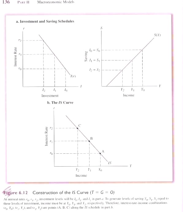
(6.9)     I(r) = S(Y)

that is, investment as a function of the interest rate (negatively sloped) equals savings (positively sloped) as a function of income (Fig. 6.12).  At a given level of r, there is a corresponding level of investment and for that level of investment there is a corresponding level of savings associated with a specific level of Y.  Taking r from Fig 6.12(a) and Y from 6.12(b) we can plot the IS curve showing levels of r and Y at which I(r) = S(Y) as in Fig. 6.12 (c).

iii – Equilibrium

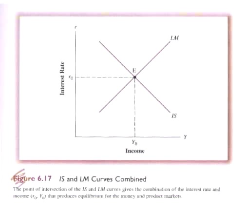
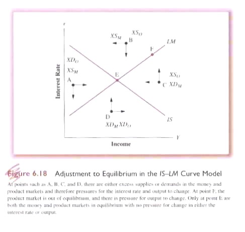
Having created the LM curve measuring the liquidity preference equilibrium given changing r and Y; and the IS curve measuring the savings/investment preference given changing r and Y we can now determine simultaneous equilibrium in the money and product markers (Fig. 6.17).  That it is an equilibrium towards which it will gravitate (assuming autonomous or exogenous factors are constant) is demonstrated in Fig. 6.18.