MACROECONOMICS +
3.0 Model
3.2 The Keynesian Model (cont'd)
(f)
LM/IS Model
1. Money Market Equilibrium
i)
Slope of the LM Curve
ii)
Shift of the LM Curve
2. Product Market Equilibrium
i) Slope of the IS Curve
ii) Shift of the IS Curve
In effect Keynes introduced three new ways of looking at the macro-economy. The first is Aggregate Expenditure: Y = C + I +G +X - Z. The second concerns money and interest and comes to fruition in the LM/IS Model. The final facet of the Keynesian Model is Aggregate Demand & Aggregate Supply.
The LM/IS Model is the Keynesian method to determine simultaneous equilibrium in the commodity (output) and money market, two assumptions must be made:
· policy variables are assumed fixed, i.e., Ms, G, T; and,
· other autonomous or exogenous factors are assumed fixed, e.g., business expectations about investment.
Keynesian demand for money includes,: transactional, precautionary and speculative demand components. It will continue to be assumed that precautionary demand is a form of ‘unexpected’ transaction demand and we are left with: transactional and speculative demand.
Transactional demand varies positively with the level of income, i.e. the higher the level of income, the higher the transactional demand. Speculative demand varies inversely with the interest rate, i.e. the higher the interest rate the lower the level of speculative demand. Transaction demand also varies inversely with the interest rate, i.e., the higher the rate of interest the greater the opportunity cost of holding cash. Accordingly, the demand for money can be generically expressed as [n.b. please note that the following equations are numbered according to the 8th Ed.] :
(7.3) Md = L(Y, r)
Alternatively, expressed in linear form:
(7.4) Md = co + c1Y – c2r where co> 0, c1 > 0 and c2 > 0
Given our assumptions, especially that the money supply is fixed expressed as Ms0, what combinations of r and Y will result in equilibrium of Md and Ms0? In linear terms:
(7.5) Ms0 = Md = c0 + c1Y – c2r
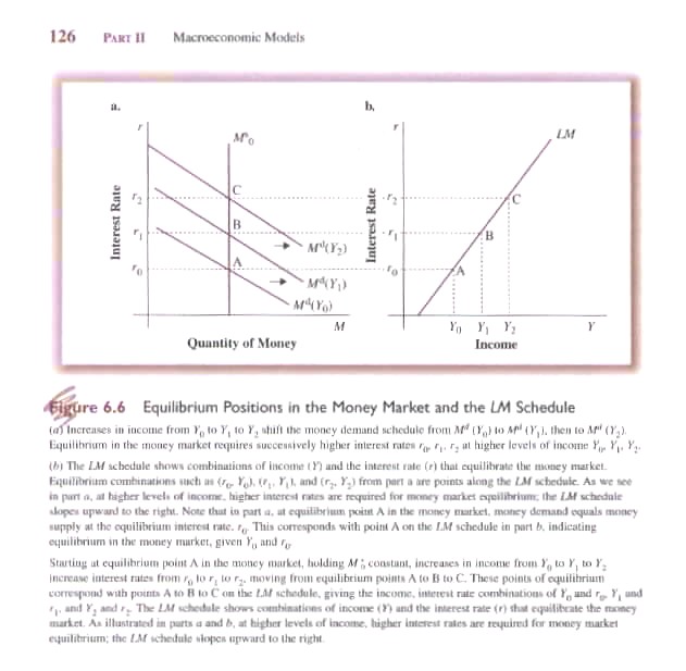
7th Ed Fig. 6.6 & 8th Ed Fig. 7.6 demonstrates equilibrium in the money market given Ms0 and different levels of Y(0, 1, 2). At Y0 equilibrium is achieved at r0. If Y increases to Y1 then transactional demand increases but with a fixed money supply this increased demand raises the price of money, i.e., the interest rate increases from r0 to r1. This increase in interest reduces speculative demand for money and also lowers the transactional demand at any given level of Y (opportunity cost increases leading to improved cash management practices reducing transactional demand). Equilibrium is re-established when the increased transaction demand resulting from an increase in Y is exactly offset by the decline in speculative and transactional demand caused by the increase in interest rates. By varying Y we can deduce a series of points (A, B, C) where, given a fixed money supply and increases in Y, a new equilibrium interest rate will exist (ro, r1, r2). These points (Y, r) can then be plotted to generate the LM curve (7th Ed Fig. 6.6b & 8th Ed Fig. 7.6b) that trace equilibrium conditions in the money market.
Two additional policy-relevant questions need be answered. First what is the slope of the LM curve – steep or gentle? Second, what causes the LM curve to shift?
The slope of the LM curve reflects the change in interest rate caused by an increase in Y, i.e. Δr/ΔY. There are two factors that affect the slope: the value of c1 and the elasticity of demand for money, specifically the value of c2.
First, from equation 7.4 we know that Md = co + c1Y – c2r. Dealing only with an increase in Y, Md will increase if Y increases by c1 times ΔY where c1 is a parameter of the increase in money demand per unit increase in income. Given a fixed money supply, the interest rate will have to rise enough to offset this income-induced increase in the demand for money. The higher c1, the larger will be the required increase in the interest rate; the smaller c1, the lower the necessary increase in the interest rate. Alternatively, the higher the value of c1 the steeper will be the slope of the LM curve. The value of c1, however, is relatively stable determined by ‘institutional factors’, e.g., payment periods and technology.
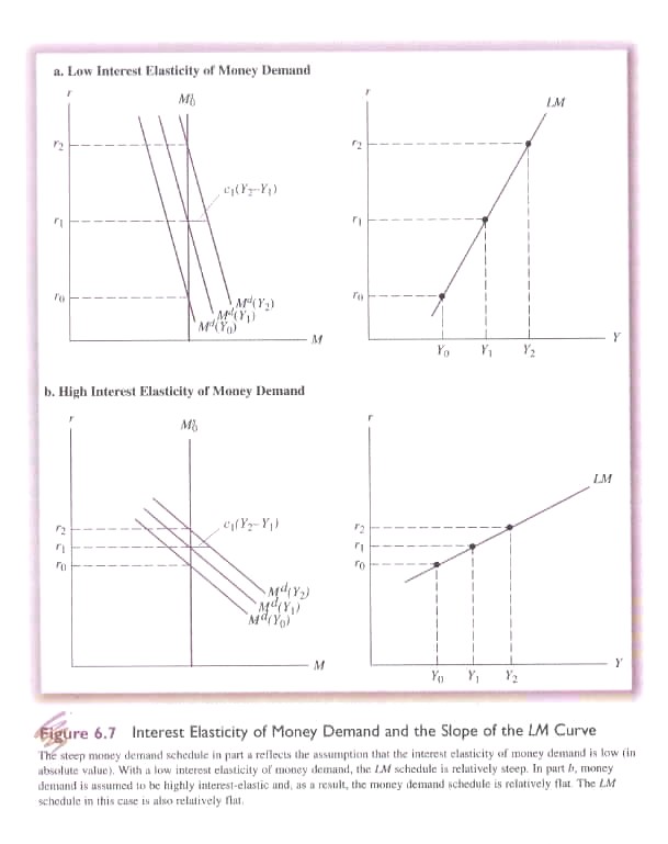
Second, dealing only with the response of Md to a change in r (or the interest rate elasticity of the demand for money) we know that an increase in r increases the opportunity cost of holding money causing a reduction in speculative and transactional demand. In equation 7.4 we know that Md = co + c1Y – c2r where c2 measures the change in Md for a change in r (-c2 = ΔMd/Δr). 7th Ed Fig. 6.7a & 8th Ed Fig. 7.7a shows Md with a very low elasticity (steep) (measured in absolute value, i.e. ignoring the negative sign associated with c2). This means c2 is relatively low meaning that a relatively small increase in Y will require a large increase in r to reduced speculative and transactional demand to compensate for the income-induced increase in Md. Alternatively if the Md is very interest-elastic (gentle) as in 7th Ed Fig. 6.7b & 8th Ed Fig. 7.7b then c2 is relatively large and only a small change in r is required.
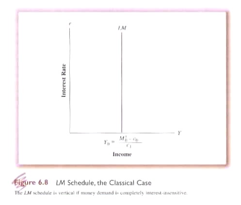
There are two extreme cases, perfectly interest inelastic and perfectly interest elastic demand for money. First, if the demand for money is perfectly inelastic relative to the interest rate then c2 = 0. In effect this means that equation 6.4 reduces to: Md = co + c1Y, i.e., the demand for money is simply a function of Y. This is the situation in the Classical Model. Accordingly, the demand for money will not change in response to changing interest rates and the LM curve will be vertical (7th Ed Fig. 6.8 & 8th Ed Fig. 7.8), or, Md = Ms0 = c0 +c1Y and:
(7.6) Y = (Ms0 – c0)/c1
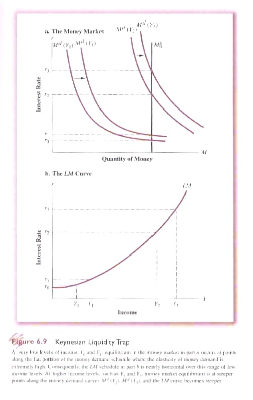
Second, if the demand for money is perfectly elastic (approaching infinity) with respect to changes in the interest rate. As noted in the discussion of speculative demand, Keynes believed that at very low rates of interest speculative demand would be very high because the opportunity cost of holding cash will be low and the danger of future capital losses high, i.e., if one buys a bond at a very low interest rate and rates then increase, the price of the bond must be reduced to generate a yield equal to the now higher prevailing rate of interest. This situation creates what Keynes called ‘the liquidity trap’ where changes in the rate of interest has little or no impact on Md. (please see: Krugman 2003) However, this situation exists only at very low levels of interest and accordingly we must change from a linear to a curvilinear expression of both Md and LM curves (7th Ed Fig. 6.9; 8th Ed Fig. 7.9). In effect this means that the slope of these curves is not constant but rather varies according to the level of the interest rate. Where and when a liquidity trap can occur is a matter of heated policy debate..
As in most economic analysis, movements along with ‘sliding’ points of equilibrium reflect change in endogenous variables, i.e., what is ‘inside’ the system and that which is plotted on the x- and y-axis. Shifts in curves reflects changes in exogenous or ‘fixed’ factors. Thus above we saw the mutual adjustment of Y and r to changes in each other including slope and elasticity. Next consider changes in two exogenous factors: a fixed money supply and a change in ‘liquidity preference’, i.e., changes to the set of ‘institutional conditions defining payment period and technology as well as ‘the climate of the times’.
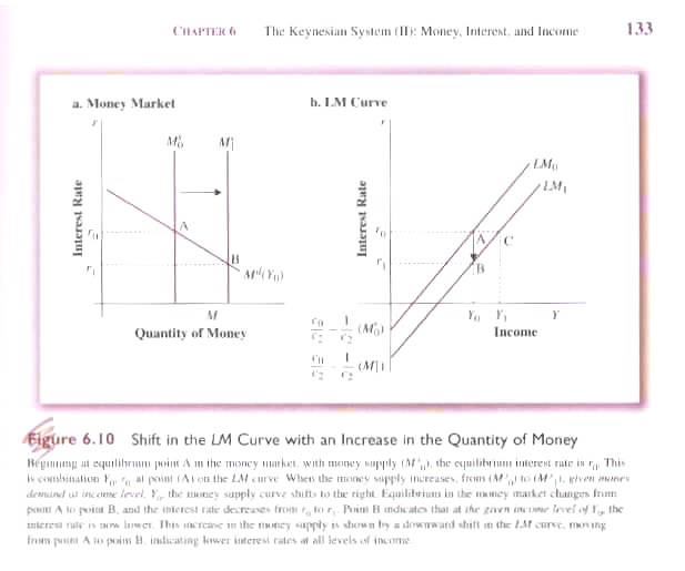
First, consider a change in the money supply Ms. It has been assumed Ms is fixed exogenously by the ‘monetary authorities’. For whatever reasons the authority changes the money supply (7th Ed Fig. 6.10; 8th Ed Fig. 7.10). We know:
(7.5) Ms0 = Md = c0 + c1Y – c2r solving for r
(7.5a)
![]()
or the LM curve with intercept c0/c2 -1/c3(Ms0)
and slope c1Y/c2.
Given the money supply (Ms0) is a component of the intercept then an increase or decrease in Ms will cause the intercept to move up or down. Furthermore, because of the minus sign the intercept will move in the opposite direction, i.e., an increase in Ms causes the intercept to drop (7th Ed Fig. 6.10; 8th Ed Fig. 7.10). If Y is fixed, then an increase in Ms means more money is held as cash at every level of interest. If Y is allowed to vary then the existing rate of interest r0 can be maintained only if Y increases from Y0 to Y1.
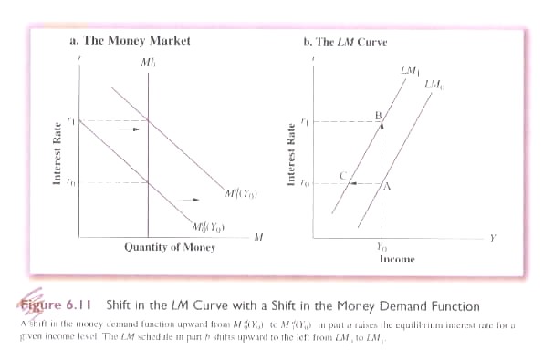
Second, consider a change in the money demand function: Md = c0 + c1Y – c2r. We have seen that the parameters (c0, c1 & c2) are established in an institutional manner, i.e., routinized patterns of behaviour. If everyone is confident that today will continue smoothly into tomorrow these parameters will tend to remain relatively constant. But if confidence breaks down then their values will tend to change. If there is concern about a significant increase in interest (and the accompanying concern about capital losses) there will be a tendency to hold more money, i.e., at every current rate of interest more money will be held shifting the Md up to the right (7th Ed Fig. 6.11; 8th Ed Fig. 7.11). In response the LM curve, at each rate of interest, will tend to shift to the left reflecting a greater demand for liquidity at each interest rate. Similarly, if there are changes in the payment habits and technology there can be a change in the amount of money held at each interest rate, e.g., introduction of POS systems and debit cards reduce the amount of money held at each interest rate reflecting better ‘cash management’.
Hidden behind the scenes of the model, unseen things are happening. Everyone is planning what to do tomorrow. Futurity and expectations rule! There are shopping lists, schedules of the marginal efficiency of corporate investment and government projects or missions that could be activated. There are contingency schedules for events in declining probability of occurrence. Matrix after matrix of numbers cascades endlessly down countless unnumbered screens in thousands and thousands of offices, factories, departments and agencies in hundreds of countries around the world. Scenario after scenario is played out or bargained between corporate and/or public peoples and computers from many cities, towns, regions and/or nation states. Odds are counted up and then counted down. The well-being of our companies, our communities, our culture hangs in the balance while the vision of a single shared planet remains hidden in the mists of immediacy.
But then, of course and inevitably, a ‘realized’ future never matches our expectations nor our preferred future and we must begin again until, finally and simply, we assume that equilibrium in the product market occurs when:
(7.7) Y = C + I + G, or, alternatively,
(7.8) I + G = S + T
Assuming, for the moment, that there is no government sector we can simplify the equilibrium condition as:
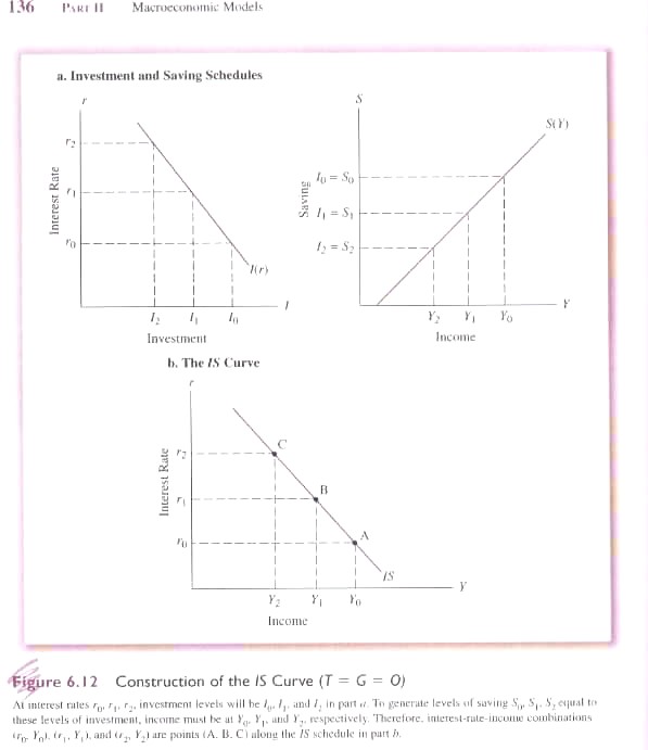
(7.9) I(r) = S(Y)
that is, investment as a function of the interest rate (negatively sloped) equals savings (positively sloped) as a function of income (7th Ed Fig. 6.12; 8th Ed Fig. 7.12). At a given level of r, there is a corresponding level of investment and for that level of investment there is a corresponding level of savings associated with a specific level of Y. Taking r from 7th Ed Fig 6.12a & 8th Ed Fig. 7.12a and Y from 7th Ed Fig. 6.12b & 8th Ed Fig. 7.12b, we can plot the IS curve showing levels of r and Y at which I(r) = S(Y) as in 7th Ed Fig. 6.12c & 8th Ed Fig. 7.12c.
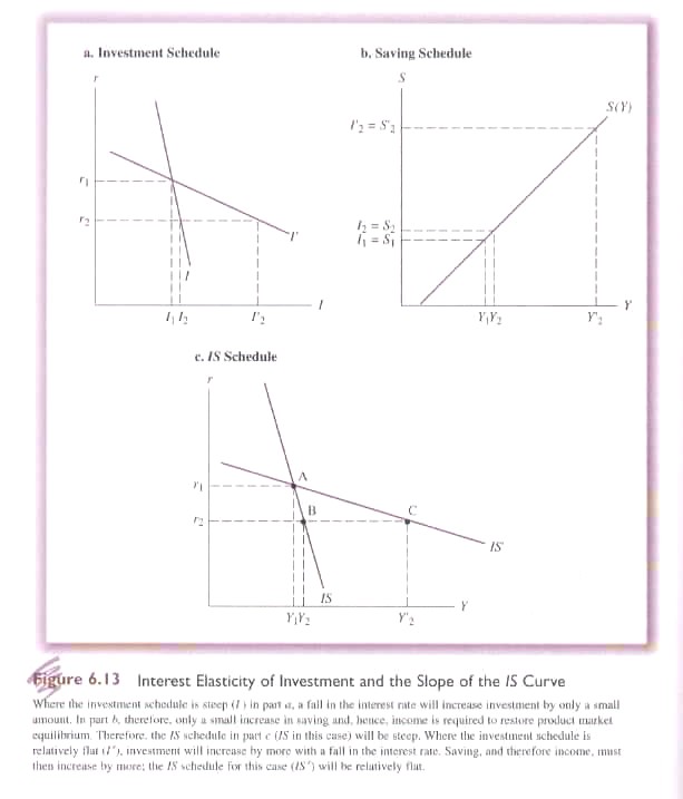
Two factors determine the slope of the IS curve: the interest-elasticity of investment demand and the marginal propensity to save. If investment is very responsive to changes in the interest rate then the slope of the investment function will tend to be gentle as shown in I’ in 7th Ed Fig. 6.13a & 8th Ed Fig. 7.13a. The interest elasticity of investment is relatively high compared to I. Therefore the slope of the IS curve will be steeper the lower the interest-elasticity of investment demand and gentler the higher the interest-elasticity of investment.
The marginal propensity to save (the inverse of MPC) determines the slope of the savings function (7th Ed Fig. 6.13b & 8th Ed Fig. 7.13b). The higher the MPS, the steeper the savings function. Relatively speaking the MPS is an institutional constant that does not vary in this simplified approach.
The first factor that can cause the IS curve to shift is a change in the investment function. At a given point in time business has a marginal efficiency of investment schedule that tells it the cut off point for project investment at any level of r. If the marginal efficiency of investment changes, however, for example new technologies increase the anticipated rate of return of projects then the investment schedule must be recalculated resulting in a shift in the IS curve to the right reflecting the increased level of investment at each possible level of r.
The second factor that can shift the IS curve is government spending and taxing. If we now introduce the government sector then the equilibrium conditions change to:
(7.10) I(r) + G = S(Y-T) + T
Thus savings is no longer a simple function of income but a function of ‘disposable income’. Put another way private savings (a function of disposable income) is complemented by ‘forced savings’ in the form of taxes. Similarly, private investment is complemented by government spending paid through taxes (or forced savings).
To derive the IS curve with an active government sector we begin with the investment function that is downward sloping with respect to the interest rate complemented by government spending which is autonomously determined (7th Ed Fig. 6.14a & 8th Ed Fig. 7.14a). Similarly, the savings function is shifted to right by the amount of taxes subtracted from gross income. In both cases G and T are assumed autonomous ‘fixed’ amounts that do not vary, in the first instance (G) with the interest rate, and in the second (T) with income. Using the two modified curves [(I+G) and S(Y-T)] we can calculate the level of interest at which investment will equal savings and the corresponding level of income to plot the IS curve (7th Ed Fig. 6.14 & 8th Ed Fig. 7.14).
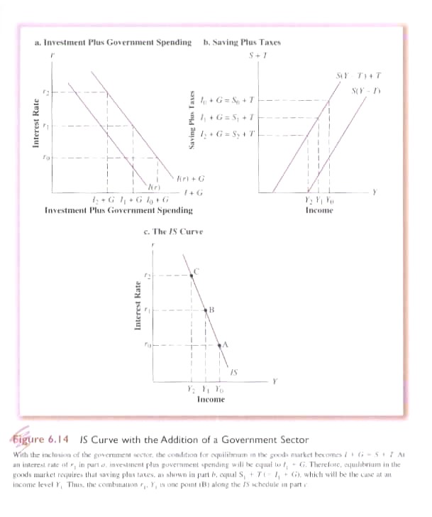
Having reached equilibrium government, as an autonomous player, can decide to change G or T. What will be the effect?
First, if G is increased the combined I + G curve shifts to the right (7th Ed Fig. 6.15a & 8th Ed Fig. 7.15a). Equilibrium will require an equally higher increase in S + T that can only be provided if Y increases from Yo to Y1 (7th Ed Fig. 6.15b & 8th Ed Fig. 7.15b). Assuming G does not crowd out I (i.e. government borrowing on the bond market) then the existing rate of interest (r0) can be maintained if Y so increases. This means at each level of interest the IS curve shifts to the right from IS0 to IS1 and at r0 from Y0 to Y1. But what is the relationship between ΔG and ΔY? It will be:
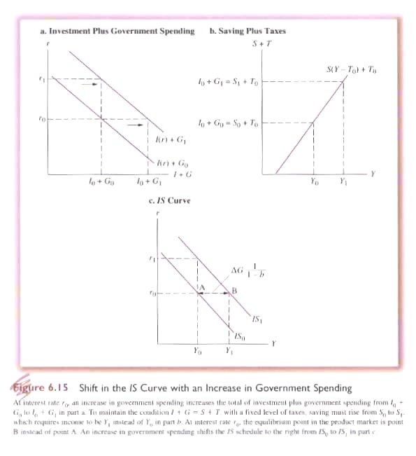
(6.11) ΔYr0 = ΔG(1/1-b) where 1-b equals the MPS, or rather, 1 minus the MPC and (1/1-b) is the autonomous expenditure multiplier Eq. 5.21.
Second, what happens if T changes. A tax increase does not directly affect the investment function (7th Ed Fig. 6.16a & 8th Ed Fig. 7.16a). Instead it cuts into savings shifting the savings function to the left (7th Ed Fig. 6.16b & 8th Ed Fig. 7.16b). To maintain the existing rate of interest (r0) Y must decrease from Y0 to Y1. This shifts the IS curve to the left (7th Ed Fig. 6.16c & 8th Ed Fig. 7.16c). Again, by how much? By the tax multiplier (Eq. 5.22) or ΔYr0 = ΔT(-b/1-b).
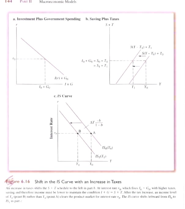
Finally, we know that investment confidence and expectations can change (autonomous change in the investment function). What will be the effect of an increase in confidence? If we take 7th Ed Fig. 6.15 & 8th Ed Fig. 7.15 and replace ΔG with ΔI, we have the same effect. That is, the I+G function shifts to the right and income must grow if the existing rate of interest (r0) is to be maintained and the IS curve will shift to the right. And by how much, by the autonomous expenditure multiplier: ΔYr0 = ΔI(1/1-b)
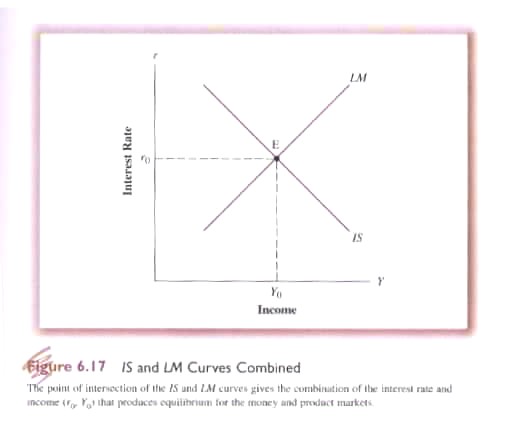
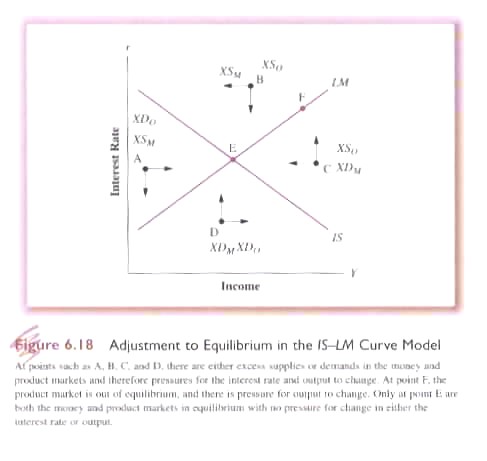
Having created the LM curve measuring the liquidity preference equilibrium given changing r and Y; and the IS curve measuring the savings/investment preference given changing r and Y we can now determine simultaneous equilibrium in the money and product markers (7th Ed Fig. 6.17 & 8th Ed Fig. 7.17). That it is an equilibrium towards which it will gravitate (assuming autonomous or exogenous factors are constant) is demonstrated in 7th Ed Fig. 6.18 & 8th Ed Fig. 7.18.