|
MACROECONOMICS + 3.0 Model 3.4 The New Classical Model |
|
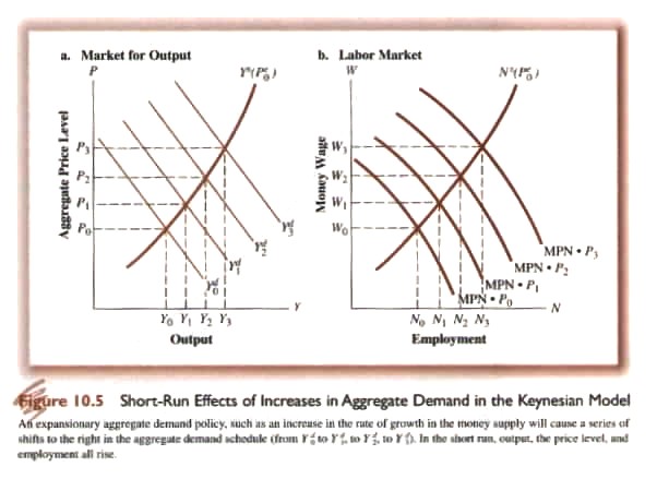
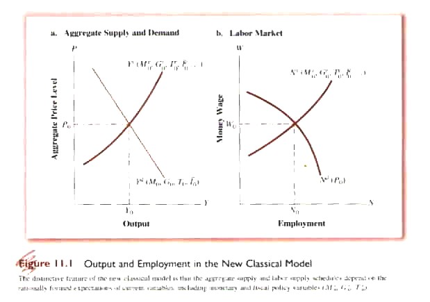
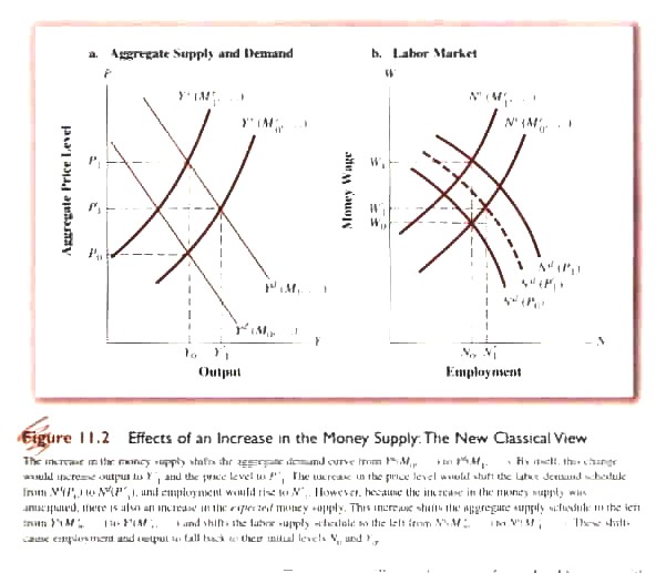
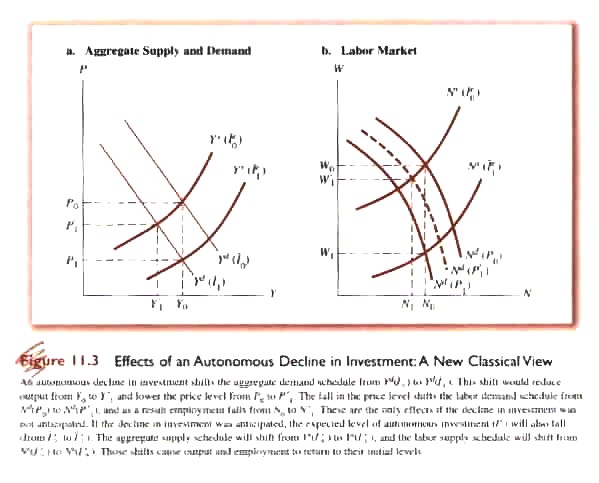
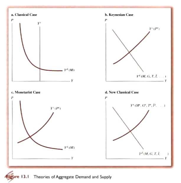
In the Keynesian Model (and to a lesser extent in the Monetarist Model) it is assumed that price expectations of labour, i.e., the future of prices, tend to react slowly in response to past experience (Eq 8.6). In effect, this amounts to backward looking expectations or projection into the future of past experience with current experience absorbed over time. Due to this lag on the part of labour the aggregate supply curve is assumed to be upward sloping in the short run. The policy implication, e.g., of an increase in the money supply, can be seen in Fig. 10.5. The increase in M shifts the aggregate demand curve (ADC) up to the right as in Fig. 10.5b (why: increased M causes r to decline resulting in I increasing). As the ADC shifts both output (Y) and prices increase (P). Given the lag in labour price expectations as prices rise employers earn a higher profit (assuming Wm remains fixed in the short run) and increase employment (Fig. 10.5b). The New Classical Model (or the School of Rational Expectations) does not accept the Keynesian and Monetarist assumption about backward looking expectations. Rather it assumes forward looking or rational, i.e., there will be no systematic error in expectations. Expectations are assumed to be made based on all available information concerning any variable being predicted and economic agents, e.g., workers, use such information intelligently, i.e., they understand how changes in the variable being predicted will affect other variables. If this is the case then labour will not suffer a lag in price expectations. This assumes, of course, that economic agents can in fact predict changes, e.g., policy changes. If they cannot predict changes then the outcome will be closer to that proposed by the Keynesian and Monetarist Models. Taking the case of labour (a similar analysis can be done for other economic agents), in the New Classical Model the supply of labour would be: (11.1) Ns = t(W/Pe) where t is a given time period, W is the money wage and Pe is price expectations The implication is that the aggregate supply curve (ASC), based on the interaction of the demand and supply of labour (assuming all other factors of production and their prices are held constant) will depend on expected rather than historical prices. In the New Classical Model in fact Pe depends on the expected level of all components of the model, i.e., Me, Ge, Te, Ie, etc. This is demonstrated in Fig. 11.1. In this Model assume the money supply is increased. If the increase in the money supply is expected (Fig. 11.2) the shift of the ADC (from Y1 to Y0) will be offset because labour will not accept the existing money wage and require a higher one shifting the supply curve of labour (N1 to N0) to compensate for the expected rise in prices. In turn, the ADC will shift back from Y0 to Y1 and the only change will be higher money wages and prices (leaving the real wage unchanged) but no increase output (Y). If the increase in the money supply is not expected (monetary surprise), however, then the ADC will shift up to the right from Y1 to Y0 (Fig. 11.2). If it were not expected then labour would initially accept the existing money wage and the demand curve for labour would shift (NdP0 to NdP1) as prices increase (Fig. 10.5). Thus, in the short run, an unanticipated increase in the money supply will have an affect on output. In the long run, however, as the price level rises labour begins to demand a higher money wage and the supply curve of labour will shift up to the left and there will be no long run increase in Y but money wages and prices will rise. Thus the New Classical Model differs from the Keynesian with respect to anticipated or expected change but not with respect to unexpected or unanticipated change. The New Classical Model does not differ from the Classical Model with respect to anticipated change but does differ in that there is no assumption of ‘perfect knowledge’, i.e., the unexpected can cause changes in output. To this point in the New Classical Model it would seem that if government wants to direct the economy it must do so by surprise. In fact, it cannot do so in the long-run. Take the case of an unanticipated increase in government spending in response to a decline in private investment (Fig. 11.3a). The initial decline in I cause the aggregate demand curve (ADC) to shift down to the left. Output (Y) then declines from Y0 to Y1. The price level (P) also declines from P0 to P1. At a lower price level labour demand also falls (Fig. 11.3b). Additional effects depend on whether the decline in I was anticipated. i – Anticipated If anticipated then labour realizing prices are going down know that the real wage at current money wage will go up and the supply of labour will shift downward. In turn this shift the aggregate supply curve downward (Fig. 11.3a) which, in turn, reduces the price level further until equilibrium is re-established at Y0 and N0. If this is the case then there is no need for government intervention. ii – Unanticipated If the decline in I was not anticipated then labour would not anticipate the decline in P and therefore not increase the supply of labour and shift the labour supply curve, i.e., the Ns curve would stay at Ns(Ie0). Output would fall to Y1 and employment drop to N1. At this point government could intervene but if its actions are anticipated there will be a lag effect on government decision – recognition, formulation, implementation, impact. If a low level of investment is now anticipated by all economic agents then the lower price level will set in and labour will increase the supply of labour (in response to the expected higher real wage). The ASC will shift and adjustment will take place without government intervention. Thus in the case of the New Classical Model it is not fiscal intervention but stabilization that government should pursue, i.e., set clear expectation of its actions so other players can react. |