MACROECONOMICS +
3.0 Model
3.2 The Keynesian Model
The Classical Model assumed that aggregate supply would always equal aggregate demand, in essence, because of Say’s Law: supply creates its own demand. While in the mid- 19th century to the late 1920s there had been a series of ‘depressions’ – extended troughs in the business cycle – they had not lasted long enough in any one country nor embraced all countries at the same time. Prior to WWI it can in fact be argued that the level of ‘globalization’ was in fact greater than even today but it was characterized by a significantly greater ‘division of labour’. Thus ‘industrial’ manufacturing tended to concentrate in western Europe and the United States while the rest of the world served essentially as a source of raw materials and markets for goods manufactured in the ‘developed’ countries. The ‘mercantilist’ policies of the European colonial powers strived to ensure this division of labour.
With the Great Depression of the 1930s, however, the trough was both long (1929 to 1939) and extensive, i.e. the entire world suffered. The productive capacity of the developed nations in effect vastly exceeded the demand for their manufactured output. Similarly, much of agriculture and the other primary industries around the world had an enormously greater output than demand. Unemployment (of labour and other factors of production) was so great that political revolution was in the air.
It soon became clear that the Classical Model’s confidence in the equilibrating power of perfect price and wage flexibility was misplaced. Large scale industrial enterprise and industrial trade unions both presented rigidities to the automatic re-establishment of full employment and output. The change in industrial structure was highlighted in Gardiner Means and Adolf Berle's path breaking text The Modern Corporation and Private Property in 1932. Something had to be done but what? John Maynard Keynes offered the answer for the ‘liberal democracies’ in his General Theory of 1936; Mussolini, Hitler, Stalin and Tojo offered an alternative answer for totalitarian states around the world.
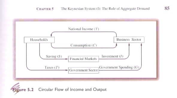
We begin our analysis of the Keynesian Model with the simplifying assumption (7th Ed. Fig. 5.2; 8th Ed Fig. 6.2; n.b. the following equations are numbered according to the 8th Ed) that:
· all factors of production (K, L, E, N where N stands for natural resources) are owned by ‘households’ (not atomistic ‘workers’ as in the Classical Model);
· all output is produced by private sector firms, i.e. there are no ‘cottage industries’ and government buys from private firms and does not produce any output itself;
· the economy is ‘closed’, i.e. there are no imports or exports, and there is therefore no difference between GDP and GNP. Furthermore, National Income (income earned by factors of production) is therefore equal to GDP (purchases of current goods and services); and,
· the aggregate price level is fixed and therefore all variables are ‘real’ and all changes are ‘real’ changes.
A central objective of the Keynesian Model is to insure that aggregate output (Y standing for supply) equals aggregate expenditure (E standing for demand), i.e.
(6.1) Y = E
In this simplified world, there are three types of demand: consumption (C), investment (I) and government spending (G). Accordingly in equilibrium:
(6.2) Y = E = C + I + G
Unlike other expenditure items that are ‘earned’ one way or another, (C by the provision of factors of production by households to firms and I by subsequent borrowing from households and paying interest), government spending (G) is financed by taxes (T) that, assuming a balanced budget, will equal G. In this sense taxes are considered a forced expenditure by households. Given this and the assumption that national product (Y) equals national income, we can say that an identity exists between output and all forms of expenditure, i.e.:
(6.3) Y
![]() C + S + T
C + S + T
One of the key concepts of the Keynesian models is ‘expectations’, i.e. decision are taken today in anticipation of conditions that will exist tomorrow. J.R. Commons introduced a similar concept called ‘futurity’, i.e. people live in tomorrow but act today. The concept of expectations is critical because it allows the Keynesian Model to handle the discrepancy that can (and usually does) occur between planned and actual or ‘realized’ outcomes. While such a discrepancy affects all expenditure items – C, I and G – Keynes placed special emphasis on the difference between planned (I) and actual or realized investment (Ir) by private firms. With this concept in mind we can say that:
(6.4) Y = C + Ir + G
By netting out common terms in Equations 5.3 and 5.4, we can conclude that:
(6.5) S + T = I + G
Similarly using Equations (6.2) and (6.4) we can conclude that in equilibrium:
(6.6) Ir = I
As we will see later in this course, the mechanism whereby realized investment is always equal to planned investment is business inventories in the Keynesian Model. (This assumption is, however, under question at present because of the recent dot.com bubble and the potential role of changes in physical capital rather than in inventories.)
There are, given our assumptions, three alternative ways of expressing equilibrium in the simplified Keynesian Model:
(6.2) Y = C + I + G
(6.5) S + T = I + G
(6.6) Ir = I
Let us quickly examine the implications of these three equilibrium conditions. First, Equation 6.2 implies that production of Y generates an equivalent level of income for households. Part of this income returns to firms: directly through the purchasing decisions of consumers (C); indirectly through the investment of consumer savings by firms; and, indirectly through the purchases of goods and services from firms by government (G) that is financed by taxes levied on households.
Second, Equation 6.5 implies that leakages from direct consumption (S +T) are exactly offset by injections (I + G) [(7th Ed. Fig. 5.2; 8th Ed Fig. 6.2]
Third, Equation 6.6 implies that planned and realized investment must be equal in equilibrium through the mechanism of adjustments in business inventories. If C + G are less than expected then business inventories will build up; if C + G is greater than expected business inventories are run down. To understand how planned and realized inventory invest can differ consider the case where:
(6.7) Y > E
C + Ir + G > C + I + G
Ir > I
In this case, actual inventories are larger than planned. Alternatively, consider the case:
(6.8) E > Y
C + I + G > C + Ir + G
I > Ir
In both Equations 6.7 and 6.8, firms will change their output decisions for the next planning period. If there are higher than desired inventories, output will fall; if there are lower than desired inventories, output will increase. The question remains: what is the desired level of inventories? This question in the Keynesian Model is answered by the experience of firms over many time periods. They learn that a certain level is optimal to allow for fluctuations in demand.
As we have seen aggregate demand in the Keynesian Model is made up of three components:
i - consumption (C);
ii - investment (I); and,
iii - government spending (G).
i – Consumption
Consumption accounts for 60 to 70% of aggregate demand. Keynes believed consumption was a stable function of disposable income, i.e. after tax income (YD = Y-T) where “T” represents ‘net taxes’, i.e. taxes minus transfers from government, e.g. UI payments. Other factors can influence consumption, e.g. expected increases in income or wealth as well as expected price changes. Such factors are not, however, generally considered significant. In summary, consumption is ‘induced’ by changes in the level of income, i.e. if income goes up C goes up and visa versa.
In the Keynesian Model the consumption function can be expressed as:
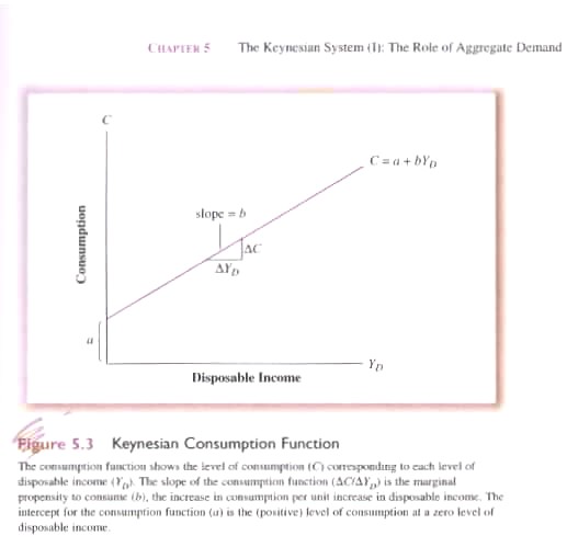
6.9 C = a + bYD where
a > 0
0 < b < 1
With respect to the terms of the consumption function: “a” represents ‘non-discretionary’ consumption or ‘survival’ spending. Thus even if you earn no income you still must eat and satisfy ‘survival requirements’, clothing, shelter etc. And how is this possible? One way is by selling off one’s assets; the other borrowing from friends or family. Non-discretionary consumption is visible in 7th Ed Fig. 5.3 and 8th Ed Fig. 6.3 as the intercept of the consumption function with the x-axis; and, “b” represents the marginal propensity to consume (MPC) or the slope of the consumption function relative to disposable income.
6.10 b = ΔC/ΔYD
It measures the increase in consumption from a unit increase in disposable income. Keynes assumed that any increase in disposable income YD would be split between consumption and savings, i.e. the increase in consumption would be less than the increase in YD. It is important to note that for individual households MPC varies according to income level. Thus the rich have a lower MPC than the poor. For the economy as a whole, however, an overall MPC can be calculated.
To sum up, it is assumed in the Keynesian Model that disposable income forms an accounting identity with consumption and savings as follows:
Given:
(6.3)
![]()
then:
(6.11)
![]()
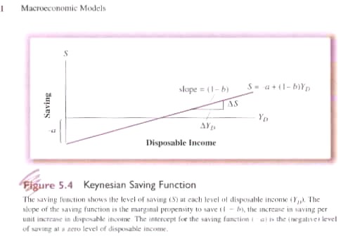
Through manipulation we can also establish the savings function (Fig. 5.4) as:
(6.12) S = -a + (1-b)YD
and the marginal propensity to save (MPS) , i.e. the increase in savings for a unit increase in disposable income as
6.13 ΔS/ΔYD = 1 – b
ii - Investment
For Keynes the change in the desired level of investment (I) by firms was a critical variable in insuring Y = E. While C was considered an induced variable by Keynes (induced by changing Y), he considered I an autonomous variable that changed not in response to ΔY but for other reasons. The two dominant factors in determining the level of I were the interest rate (r) and expected business condition, i.e. the expectation of earning a profit (π). The interest rate measured the direct or indirect cost of financing a project, i.e. investing. The anticipated profit to be earned was calculated relative to the cost of funds that must be paid to undertake the project. Given that an investment in a new plant may have to produce output for 20 or 30 years there are great uncertainties concerning investment. Some uncertainties are subject to ‘probabilistic calculation’; other, however, are what Keynes consider ‘true uncertainty’, i.e., there are risks involved. It was the willingness to accept these risks that Keynes’ summed up as ‘animal spirits’. Needless to say, such ‘spirits’ are fickle.
iii – Government Spending and Taxes
As with I, Keynes assumed that government spending and taxation were not direct functions of income, i.e. they are autonomous not induced variables of Y. Both are in fact ‘political’ variables and hence not necessarily related to ensuring Y = E.
We now have the necessary components to determine the equilibrium level of income. We begin with:
(6.2) Y = E = C + I + G
Y is the endogenous variable to be determined. Autonomous or exogenous variables: I, G & T are given from outside the model. Consumption, for the most part, is dependent or induced by changes in disposable income, i.e.
(6.9) C = a + bYD or
C = a + bY – bT
Substituting Equation 5.9 in 5.2, we get:
(6.14)
![]()
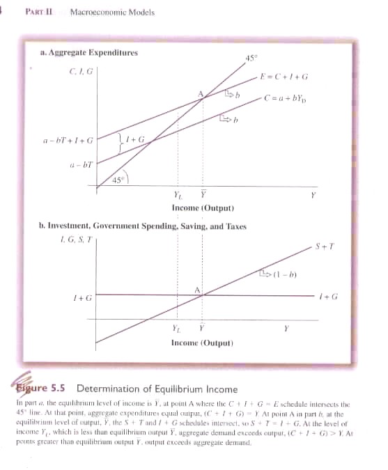
In 7th Ed Fig. 5.5 and 8th Ed Fig. 6.5 we can see the resulting curve. On the x-axis we measure Y. Along the y-axis we measure components of aggregate demand (C, I, G). When we plot the consumption function we have an upward positively sloped curve that intersects the y-axis at the level of non-discretionary consumption (a-bT). The slope of the curve is the Marginal Propensity to Consume (MPC = b) reflecting how much of income will be spent on consumption, and, by deduction, how much will be saved and available for investment purposes.
If we add autonomous aggregate demand (I, G) they simply shift the consumption function up vertically by the exogenously determined value of I and G. The slope of the resulting Aggregate Expenditure Curve (AEC) remains the same as the Consumption Curve. I and G do not vary with Y.
A 45 degree line from the origin marks all points where Aggregate Expenditure equals output. The intersection of AEC and the 45 degree line indicates where equilibrium will be achieved (A in 7th Ed Fig. 5.5 and 8th Ed Fig. 6.5). Any point above A and the AEC indicates that demand exceeds output and business inventories will be run down forcing the system back to equilibrium. Any point below A and the AEC indicates that aggregate demand is less that existing output and inventories will be built up forcing the system back into equilibrium.
From Eq. 6.2 we know that Y = E = C + I + G, i.e., E = C + I + G. Replacing C using Eq. 5.9 we know E = a + bY – bT + I + G. Put another way: E = a – bT + I + G + bY where (a-bT +I + G) is the autonomous components of expenditure and the intercept while b is the slope of the curve, a coefficient of Y equal to the MPC. Every time an autonomous expenditure changes, Aggregate Expenditure will shift, vertically, by an equal amount reflected in the change of intercept.
Equilibrium aggregate demand, however, will change by an amount greater than the change in autonomous expenditure. The first indication becomes visible by comparing the vertical change in aggregate expenditure (due to a change in autonomous expenditure) with the horizontal change in equilibrium output. Due to the slope of the Aggregate Expenditure Curve the horizontal change will be greater than the vertical. How much greater?
This is where Keynes introduced one of his most important additions to economic thinking – the multiplier. In this case the aggregate expenditure multiplier. Using
(6.14)
![]()
we can separate out (1/1-b) from changes in autonomous spending (a-bT+I+G). In fact 1/1-b is the aggregate expenditure multiplier where b = MPC. If b is less than 1 then the denominator is less than 1 and when divided into 1 will generate a number (the multiplier) that is greater than 1. That is any change in autonomous spending, especially usually more unstable investment will lead to a larger change in output equilibrium.
It is important to note that in equilibrium it is assumed that I + G = S + T. If there were no government this would mean that I must equal S for equilibrium. One of Keynes criticisms of the Classical Model was that the ‘loanable funds doctrine’ was not necessarily true. On the one hand individuals might, due to fear and insecurity, hold cash without investing it. On the other, firms might be unwilling to invest as much as consumers are willing to save. This potential instability of investment lay at the heart of Keynes’ call for an interventionist government.
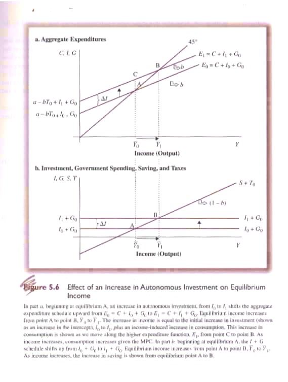
In 7th Ed Fig. 5.6 & 8th Ed Fig. 6.6 we can see the effect of the multiplier at work due to an increase in autonomous spending, specifically an increase in I. The increase in I shifts the AEC upwards by the ΔI but equilibrium output increases by more than ΔI. In effect income increases by ΔI which then increases consumption (ΔC) because part of increased Y is spent (specifically b ΔY). Therefore
ΔY = ΔI + ΔC may be expressed as
ΔY – ΔC = ΔI, and,
assuming tax
collection is fixed, then for equilibrium:
(6.19) ΔS = ΔI
Thus with T and G fixed, to restore equilibrium S must increase enough to balance ΔI. As ΔS = (1-b)ΔY and using Eq. 6.19
(1-b) ΔY = ΔI and, therefore,
(6.20) ΔY/ΔI = 1/MPS or
= 1/(1-b)
The same result will occur for ΔG. Thus,
ΔY = (1/1-b) ΔG, and,
(6.21) ΔY/ΔG = 1/1-b
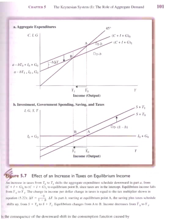
There is a difference, however, with respect to a change in taxes, i.e. ΔT (Fig. 5.7).
ΔY = (1/1-b)(-b)ΔT, or,
(6.22) ΔY/ΔT = -b/1-b
Thus an increase in T reduces disposable income causing C to fall at every level of Y (7th Ed Fig. 5.7 & 8th Ed Fig. 6.7). However, a dollar increase in T causes C to fall only by (b) with the residual (1-b) absorbed through decreased savings. Thus unlike changes in autonomous expenditure that has a multiplier effect on Y, tax change has a less than one-to-one effect. It is assumed however that changes in T are ‘flat rate changes’, i.e., a fixed amount. A somewhat different result occurs if a change is made in tax brackets. Thus if under a system of progressive taxation those who earn more pay a higher rate a change in the rate structure will have differential implications. For example lower taxes on low income earners will have a larger impact on consumption (because low income earners tend to have a higher MPC). A tax change focus on high income earners will have a greater impact on savings because high income earners tend to have a higher MPS (unless they spend on luxury goods)
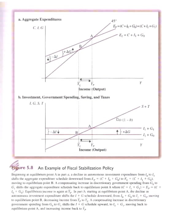
Given that changes in G or T can affect equilibrium income they can be used as conscious tools of macroeconomic policy to offset undesirable changes in I. In 7th Ed Fig. 5.8 & 8th Ed Fig. 6.8 we can see that a drop in I can be offset by increasing G.
So far we have assumed a ‘closed’ economy in which there are no exports or imports. Assuming X stands for exports and Z for imports we can specify the national income and expenditure equation as follows:
(6.23) Y = E = C + I + G + X – Z
Exports represent sales of current domestic production to foreigners. Accordingly it is part of aggregate demand. Imports, however, are purchases made from foreigners and not from current domestic production. In effect they represent a reduction in demand for domestic goods and services and are subtracted from aggregate demand.
But what is equilibrium in an open economy? We begin as before assuming G and I are autonomous of changes in Y. C , however, is induced by changes in Y, i.e.
(6.24) C = a + bY
But what determines exports and imports? Are they induced or autonomous to changes in Y? In the case of exports, demand is autonomous in that it is determined by foreign income not domestic; by the exchange rate and international prices, not domestic.
In the case of imports they depend on Y, i.e. they are induced by ΔY like C, i.e.
(5.25) Z = u + vY where
u represents the autonomous level of imports, i.e. analogous to (a)
v represents the marginal propensity to import, i.e. the percentage of additional income spent on imports
Of course if Z is induced by ΔY and C is induced by ΔY then the two are related, specifically any increase in Y will be split between consumption of domestically produce or imported goods and services. Starting with:
(6.23) Y = E = C + I + G + X – Z
And substituting : C = a + bY and Z = u + vY
(6.26) Y = (1/1-b+v)(a+ I + G + X + u)
Ignoring T, this compares with the closed economy equation
(6.27) Y = (1/1-b)(a+I+G)
The implication with respect to the expenditure multiplier is clear. The higher the propensity to import (v) the lower the multiplier. This, of course, reduces the effects of changes in autonomous expenditures, e.g. G. In effect imports act a ‘leakage’ from the system. The more leakage the less leverage is available to government, monetary authorities and domestic forces to effectively exercise macro-economic policies.