3.0 Models

After exploring the definitional complexity of contemporary macroeconomic concepts – national income accounting, national income, national income identities, GDP, disposable personal income, prices, money, growth and the business cycle - it is time to exercise what the poet Robert Frost called ‘temporary suspension of disbelief”.  We are about to move into a relatively pure exercise in deductive logic – given a set of assumptions deduce outcomes.  Like chess one has to accept the limits of the playing field – 8 x 8 – with pieces that move in specific and specified ways.  If you don’t accept the ‘rules of the game’ you can’t win!  In the case of the engines of macroeconomic analysis this means not letting reality intrude into your thinking.  In effect, economics like all professions attempts to structure thinking along a distinctive path.  It is the patterning of thought more than a precise understanding of the actual subject that is the point of the following exercise in constructing and operating the three primary macroeconomic engines of analysis – classical, Keynesian and monetarist.

To begin with before the 1930s there was no ‘macroeconomics’, i.e. the study of the overall economy rather than its constituent parts.  It is with Keynes’ General Theory [Chapter 12] that it begins, as well as the effort to deduce from the history of economic thought what were the ‘implicit’ models of previous economic thinkers.

3.1 The Classical Engine of Analysis: (a) Output and Employment

The so-called Classical School of economic thought begins with Adam Smith (1723-1790) and his An Inquiry into the Wealth of Nations in 1776 and runs through the last great Classical economist John Stuart Mill (1806-1873).  In essence the Classical School emerged as a response to the previous dominant school – the Mercantilists.  To quote Chapter One of The Wealth of Nations, the Mercantilists believed:

THAT wealth consists in money, or gold and silver, is a popular notion which naturally arises from the double function of money, as the instrument of commerce and as the measure of value.

To grow rich is to get money; and wealth and money, in short, are, in common language, considered as in every respect synonymous.

     A rich country, in the same manner as a rich man, is supposed to be a country abounding in money;

To increase the stock of money (in the form of gold and silver) Mercantilist rulers granted ‘monopolies’ to friends and relatives in order to increase domestic production of goods and services and placed severe restrictions on the import of foreign goods and services.  Such Crown grants of industrial privilege were a particular object of concern to Smith and all the Classical School that believed it was ‘real factors of production’ combined with free markets (as opposed to state-sponsored monopolies) and free trade (rather than import restrictions) that would increase the wealth of a nation defined, in essence, as the productive capacity of the economy not the quantity of money it held.  The effective collapse of the Spanish economy in spite of its enormous holdings of New World gold and silver appeared to support the Classical case. The Mercantilist and later the Bullionist view survived, however, to form the basis of what is now called the Monetarist model of the macroeconomy. 

In summary, Classical economics compared to Mercantilism:

a) stressed the role of real as opposed to monetary factors in determining real outcomes like output and employment.  Money was considered strictly a medium of exchange not a causal factor in economic growth; and,

b) stressed the role of the self-adjusting marketplace to ensure output and employment.  Government had no role in ensuring adequate demand or employment other than essential infrastructure, e.g. roads, canals and competitive markets.  In this regard, Smith noted:

People of the same trade seldom meet together, even for merriment and diversion, but the conversation ends in a conspiracy against the public, or in some contrivance to raise prices...

The interest of dealers . . . in any particular branch of trade or manufactures, is always in some respects different from, and even opposite to, that of the public ....  The proposal of any new law or regulation of commerce which comes from this order, ought always to be listened to with great precaution, and ought never to be adopted till after having been long and carefully examined, not only with the most scrupulous, but with the most suspicious attention.  It comes from an order of men, whose interest is never exactly the same with that of the public, who have generally an interest to deceive and even to oppress the public, and who accordingly have, upon many occasions, both deceived and oppressed it .

3.1.1 The Production Function

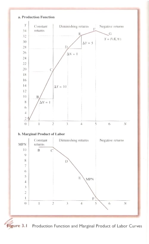
The starting point for analysis of the Classical engine  is the production function:

The Classical production function shows different levels of output (y) assuming fixed technology and varying amounts of factors of production (K = capital in the form of plant and equipment; N = labour measured in homogeneous units).   In the short-run it is assumed that the amount of capital is fixed (indicated by the symbol over K) and varying quantities of labour but assuming a fixed population (otherwise additional labour would become available simply through natural growth).

Accordingly, in the short-run, all changes in y depend upon changes in N.  The relationship is shown in Fig. 3.1. and displays a quality that is in fact derived from the Neo-Classical School or Marginalists – diminishing marginal product.  Thus the so-called Classical model is in fact a marriage of the original Classicists and the later Neo-Classicists. 

The Classical Production function (Fig. 3.1a) displays some important characteristics:

a) at low levels of N, the function is almost a straight line whose slope measures the increase in output for an increase in N.  This section of the curve reflects what are called ‘constant returns to scale’;

b) as the level of N increases, however, the slope becomes more and more gentle reflecting ‘diminishing marginal returns’, i.e. output increases proportionately less than the increase in N; and,

c)  from the production function one can calculate a related curve (Fig. 3.1b) – the Marginal Productivity of Labour (MPN). 

3.1.2 Employment

The Classical School assumed that perfect competition ruled (another Neo-Classical artifact) and that the actual quantity of labour employed would be determined by the forces of supply and demand for labour.

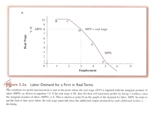
On the demand-side, a firm would hire labour up to the point at which the additional cost of a unit of labour equaled its contribution to output, i.e. until the marginal cost of labour equaled the money wage for that additional unit of labour divided by its marginal product, i.e.,

Profit maximization, in the short-run would occur when the price for a unit of output equaled MC which in turn equaled the money wage divided by the marginal productivity of the last unit of labour, or:

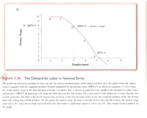
that is, profit maximization occurred when the real wage (W/P) equaled the marginal productivity of labour (measured in real terms, i.e., number of workers)

Hence profit maximization can be plotted by matching the real wage and MPN to alternative levels of N (Fig. 3.2a).    It can also be calculated in nominal terms (Fig. 3.2b).

The result is in fact a firm’s demand curve for labour and if the demand curves for all firms are added horizontally, i.e. at each real wage (or MPN), we get the aggregate demand curve for labour by all firms in the economy (N^d) are added together, or:

Eq. 3.5     N^d = f (W/P) (-)        

or, the demand for labour is a negative function of the real wage, i.e., the higher the real wage, the lower the demand for labour.

3.1.3 Labour Supply

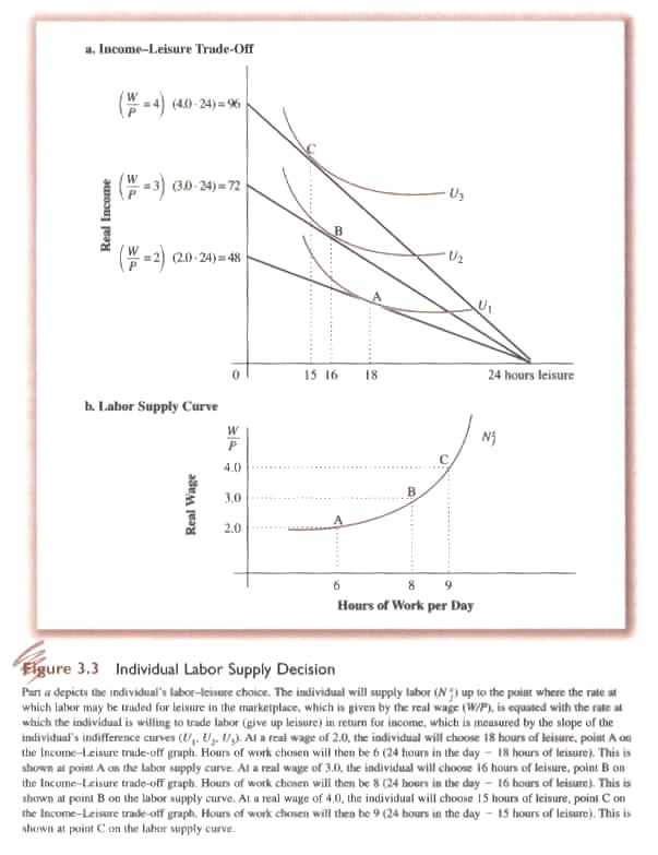
 On a daily basis, leisure is equal to 24 hours minus how much time is spent working.  Real income of worker (j) is equal to the real wage (W/P) multiplied by the number of hours worked (N^s_j).  The slope of the indifference curve shows the tradeoff a worker is willing to make between work and leisure.  In general, the higher the real wage, the more work (or the less leisure) will be chosen; the lower the real wage, the lower the amount of work supplied.  A worker will maximize utility where the budget line (rays beginning at 0 hours of work in (Fig. 3.3a) is tangent to the highest attainable indifference curve.  The higher the real wage, the steeper will be the budget line.  So at all possible levels of the real wage we can calculate how much time an individual is willing to work and, accordingly, we can plot the supply curve for labour (Fig. 3.3b).

If we horizontally sum up the hours all individual are willing to work at all possible real wages, we can calculate the economy’s supply curve of labour, or:

Eq. 3.6   N^s = g (W/P)         

or, the supply of labour is a positive function of the real wage, i.e., the higher the real wage, the higher the supply of labour..

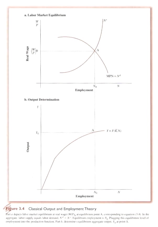
3.1.4 Equilibrium Output and Employment

To determine what the equilibrium output and level of employment will be in an economy, according to the Classical model, the supply and the demand for labour must be equal (Fig. 3.4), i.e.

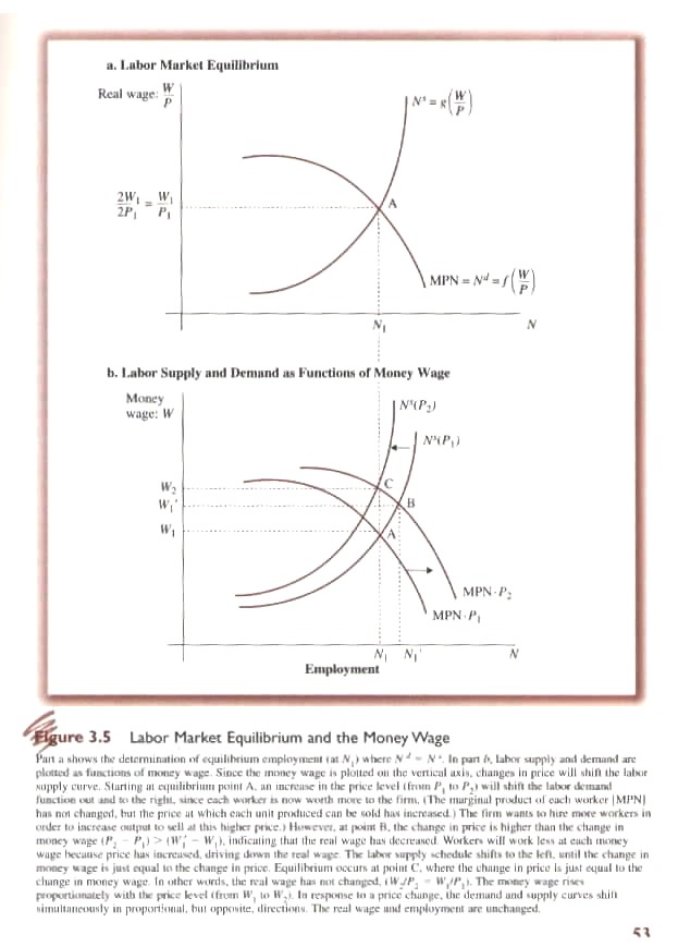
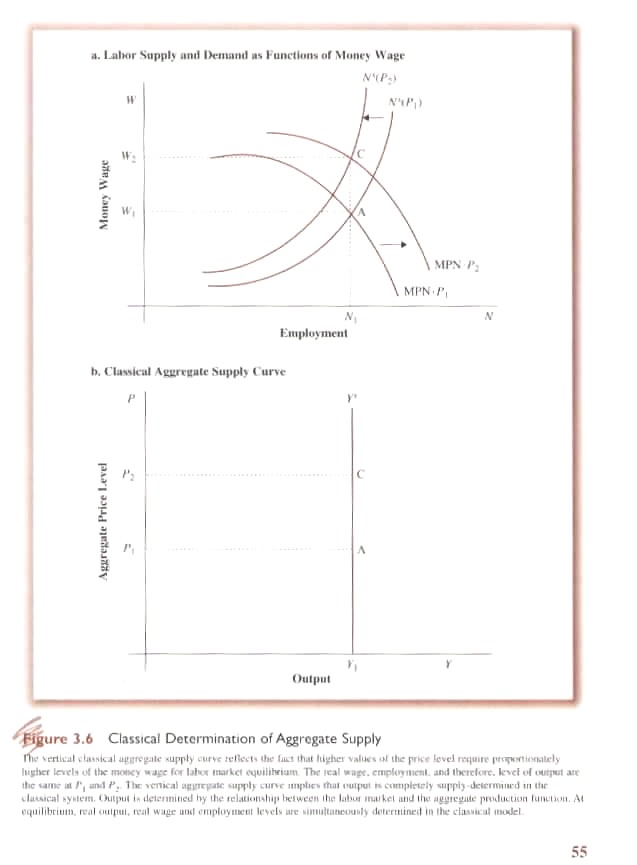
3.1.5 Determinants of Output and Employment

There are two types of variables in the Classical Model (in fact in all the models we will study).  These are endogenous (within the system – capital, labour, wage and price) and exogenous (outside the system – technology, population growth).  In the Classical system the exogenous variables affect supply rather than demand.  Thus if there is technological change then the MPN will change; if population increases or decreases the supply of labour will change.  The Classical system does not consider demand to be a question.  In effect, Say’s Law is assumed to hold:  supply creates its own demand, and, accordingly, there is never a lack of aggregate demand.

So far we have considered only the real wage rate (W/P) as playing a role.  The question arises as to what effect changes in the money wage and money price will have on output.  From Eq.’s 3.5 and 3.8 we calculate the supply and demand curve for labour (Fig. 3.5a).  If money P or W change then the real wage will change.  If the real wage changes so will the demand and supply of labour (Fig. 3.5b).  Given the money wage, a firm will choose the quantity of labour where:

Eq. 3.9   W = MPN x P or, the money wage equals the MPN times the Price of goods and services.

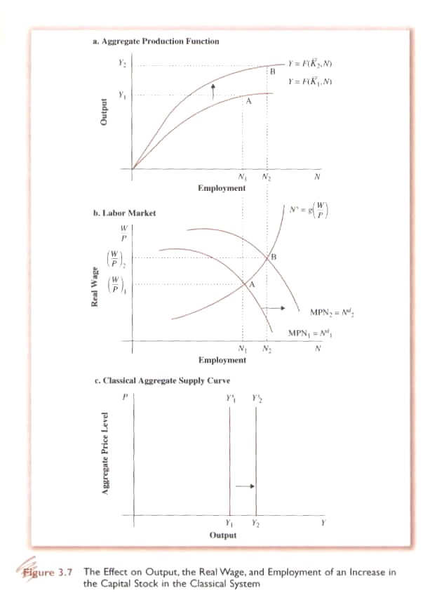
3.1.6 Factors Not Affecting Output

Because output is determined purely by supply factors under the Classical model, demand plays no role.  Similarly factors like the quantity of money, level of government spending, and demand for investment goods are all ‘demand’ factors that play no role in determining output in the Classical Model.   Taxes that affect supply-side factors will, however, affect output.

Factors affecting the Classical equilibrium include changes in technology, reduction of the price of raw materials as well as growth of the capital stock (Fig. 3.7).

3.1.7 Conclusions for the Classical Model - Output & Employment

The Classical model is thus characterized by the supply-determined nature of real output and employment.  The aggregate supply curve is vertical because of assumptions made about the labour market: (i) perfectly flexible wages and prices; and, implicitly, (ii) perfect information, and, of course, perfectly competitive industries.