1.3.4

Index

2. One Fixed Factor Cost Function

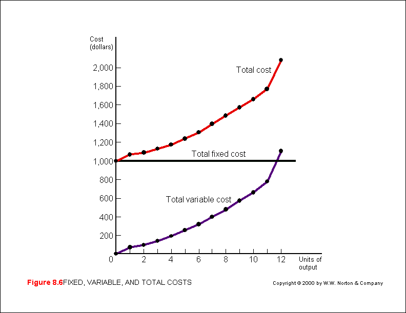
d) The Supply Curve: Shutdown & Breakeven

In the short-run at least one factor of production is fixed. During this period a firm can produce varying levels of output but only by varying variable inputs. Accordingly the firm has three distinct types of costs:

i - fixed costs associated with the fixed factor of production - usually K. Fixed costs must be paid no matter the level of output, i.e. even if the firm shuts down fixed costs still have to be paid;

ii - variable costs associated with variable factors of production - usually L. Variable costs rise and fall according to how much of the variable factors are employed. The higher the level of production, all things being equal, the higher the variable costs; and,

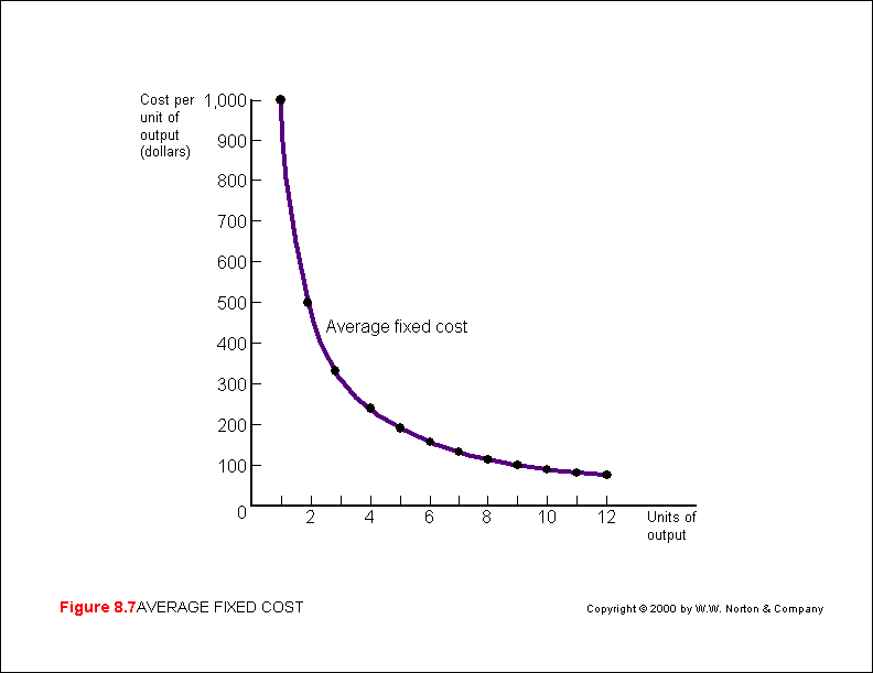
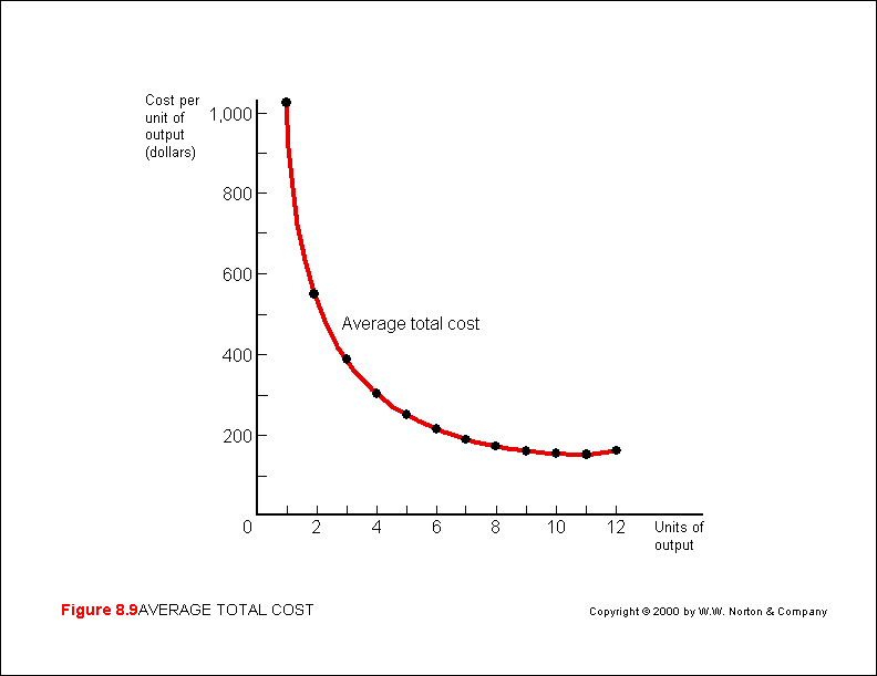
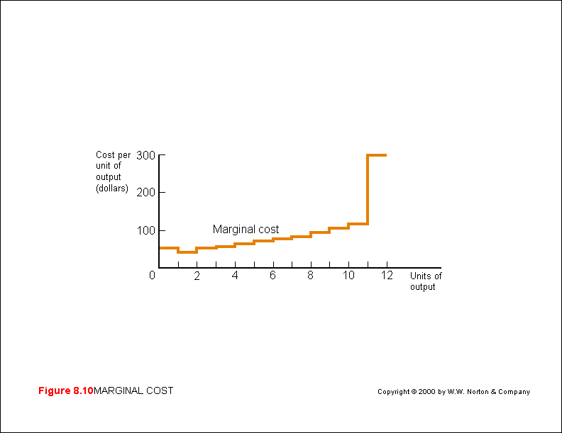
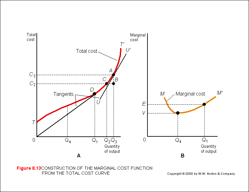
iii - total costs that include all fixed and variable costs or TC = TFC + TVC (M&Y 10th Fig. 8.6; M&Y 11th Fig. 7.7; B&B Fig. 8.13; B&Z Fig. 8.2).

In turn, for each type of cost at every level of production, average costs can be calculated:

i - Average Fixed Cost (AFC) = fixed cost per unit output (M&Y 10th Fig. 8.7; M&Y 11th Fig. 7.8; B&B Fig. 8.16; B&Z not displayed). AFC will decline as output increases as the fixed cost is spread over a larger and larger level of output;

ii - Average Variable Cost (AVC) = variable cost per unit output (M&Y 10th Fig. 8.8; M&Y 11th Fig. 7.9; B&Z Fig. 8.2). The distance between the AVC curve and the TC curve will tend to narrow as output increases because AFC declines as output increases; and,

iii - Average Total Cost (ATC) = fixed (AFC) + variable (AVC) cost per unit output (M&Y 10th Fig. 8.9; M&Y 11th Fig. 7.10; B&B not displayed; B&Z Fig. 8.2).

For each level of production, marginal cost can also be calculated from the additional cost associated with one additional unit of output (M&Y 10th Fig. 8.10; M&Y 11th Fig. 7.11; B&B not displayed; B&Z not displayed).

Average total and marginal cost can also be calculated from the total cost curve. Average total cost can be derived from the slope of a straight line or 'ray' drawn from the origin to any point on the total cost curve (M&Y 10th Fig. 8.12; M&Y 11th Fig. 7.14; B&B Fig. 8.7; B&Z Fig. 8.3). Marginal cost can be derived from the changing slope of the total cost curve itself (M&Y 10th Fig. 8.13; M&Y 11th Fig. 7.15; B&B Fig. 8.7; B&Z Fig. 8.3).

Marginal cost (MC) will initially decline as output increases but eventually, assuming at least one fixed factor of production, the Law of Diminishing Returns sets in and marginal cost begins to rise. The MC curve will cut the average cost curve (AC) at its lowest point. Thus as long as MC < AC then AC falls; when MC = AC then AC will be at its minimum; when MC > AC then AC will increase (M&Y10th Fig. 8.14; M&Y Fig. 7.16; B&B Fig. 8.7; B&Z Fig. 8.3).

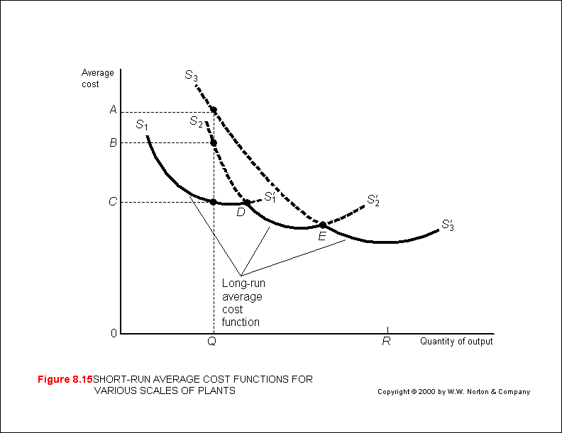
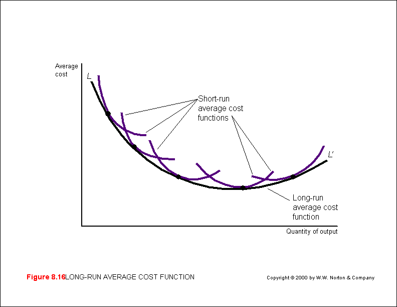
Using the one fixed factor cost function, the long-run cost or expansion path of a firm is considered to be the sequence of short-run (SR) scenarios for varying scale of plant and equipment (M&Y 10th Fig. 8.15; M&Y 11th Fig. 7.18; B&B not displayed; B&Z not displayed). In each SR scenario the scale of plant and equipment increases but during that period plant and equipment are consider to be fixed. The result is a set of average cost curve for each scale of production. An envelop curve can then be drawn representing the long-run (LR) minimum average cost at each level of output (M&Y 10th Fig. 8.16; M&Y 11th Fig. 7.19; B&B Fig 8.17; B&Z Fig. 8.7). The question remains as to when this series of SR scenarios becomes the LR.

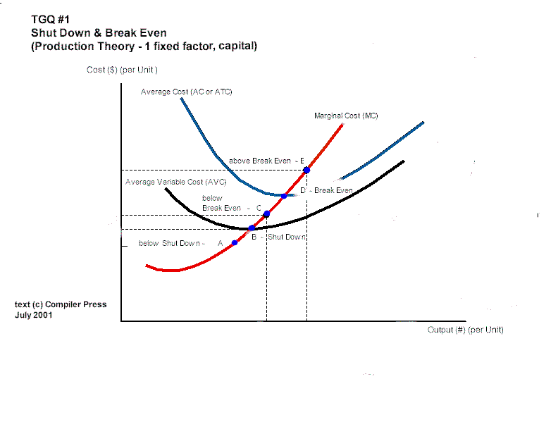
The question remains: How much output will a firm be willing to supply given its cost constraints? Put another way: What is the firm's supply curve? This depends on how much the firm can get for its output, i.e. the price or revenue it receives per unit (adjusted M&Y 10th Fig. 9.3; M&Y 11th Fig. 8.4; B&B Fig. 9.2; B&Z Fig. 9.3). If a firm cannot earn at least enough to cover all of its variable costs then in the short run it will shut down. This occurs at point B where marginal cost is equal to minimum average variable cost. This is called the 'shut down point'. If a firm earns a price higher than B it can cover all of its variable costs and some of its fixed costs and it will stay in business. Put another way, the firm will maximize profits by minimizing losses.

In the long run, however, a firm must cover all costs - fixed and variable - or it will go out of business. This occurs at point D where marginal cost is equal to minimum average total cost. This is called the 'break even point'. At this point all factors of production - including entrepreneurship - are fully paid their opportunity cost. If the firm receives a price higher than the break even point then it will earn economic or excess profits.

Thus the supply curve of a firm is the marginal cost curve above minimum AVC in the short-run and above ATC in the long-run.

It is important to appreciate that the price or revenue a firm receives applies to each and every unit of output it sells. Accordingly it will produce to the point at which the cost of the next unit of output (MC) equals the price or revenue it receives for that last unit. In effect, a firm earns a profit on each previous unit (if the price or revenue is greater than minimum AVC or minimum ATC in the short- and long-run, respectively). A firm thus maximizes its profits by producing at the point where price or revenue equals marginal cost of the last unit of output.